This lesson will teach you how to use the Vstack function to link information between tables. So that if the user adds any new item to a table, it will be added to the other table automatically.
We will put a set of “Sheets” and then create a table on each sheet containing a set of information.
Objectives of using the Vstack function
First, we make sure that all the information is in the form of tables. This is done by moving to each sheet and then pressing “Control + T” from the keyboard.
as this process has two objectives:
- First, using tables allows the use of table names in the “Formula”. We can benefit from the table names in many additional features of the table in addition to the various Excel options.
- Second, achieving our main goal, which is that any update in the tables will be automatically added to the main table located on the main sheet “Main Sheet”. If we try to write a specific phrase in Table B, which is linked to Table A. Note that the two tables are located on two different sheets. Then the same statement will be added to table A.
So, to begin with, we will go to the first sheet “Sheet 1”. Then we will select and then copy the table titles that are in it.
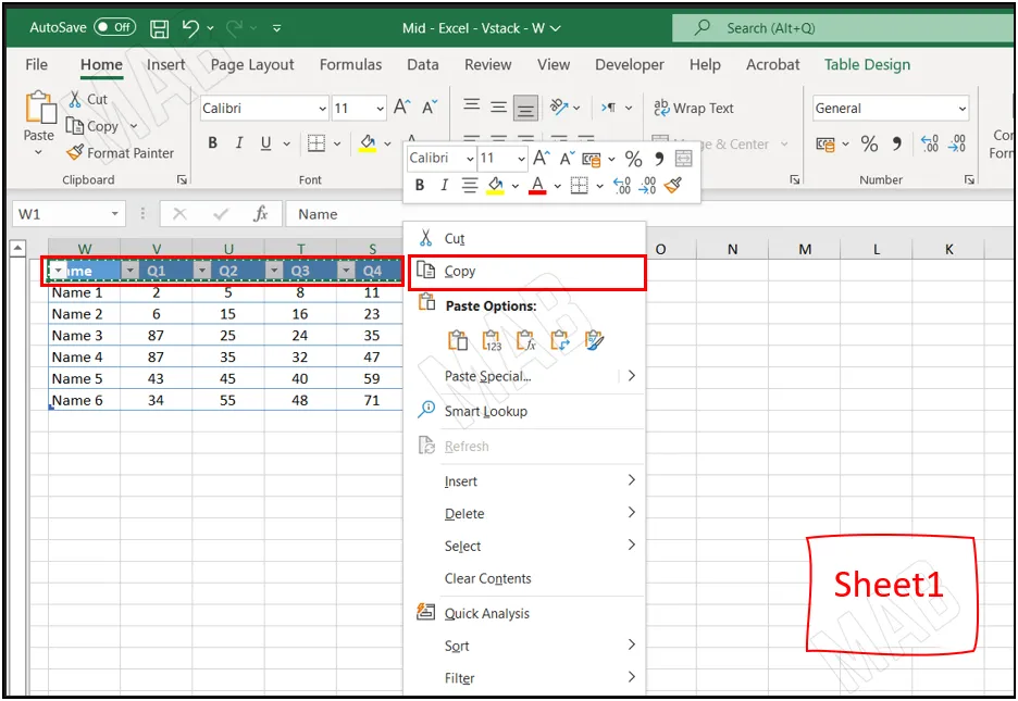
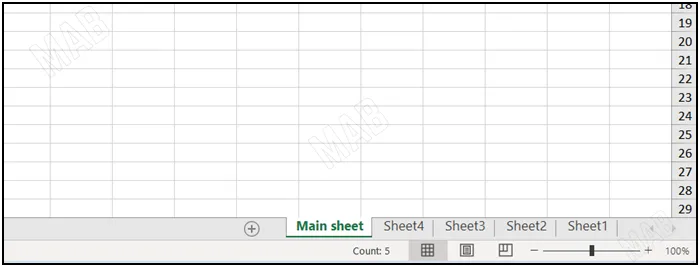
After that, we will go to the sheet that we will consider the main sheet and paste the table titles we copied.

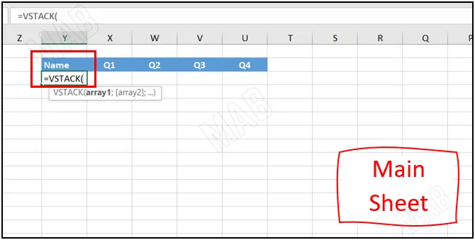
We go to the main sheet and then use a function called “=VSTACK ” by writing the function’s name.
We go to the first sheet and then select the information from the first table (without the titles). Thus, this table information will be added to become inputs for the Vstack function.
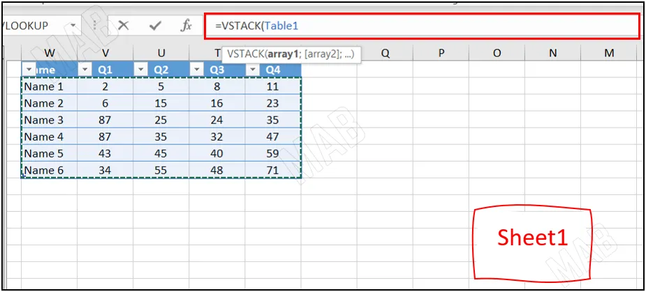
Determining the function inputs
We now have two options:
First, from the top bar, we type a comma “,” then move to the second sheet, specify its information, and so on.
Second, from the top bar, we type a comma “,” and then we continue writing the names of the tables in the rest of the sheets.
The result will be the same.
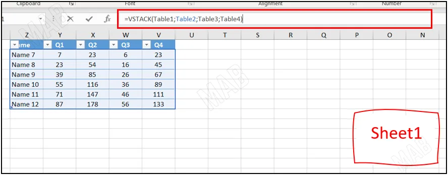
From the keyboard, we choose “Enter”.
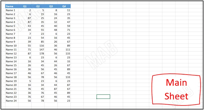
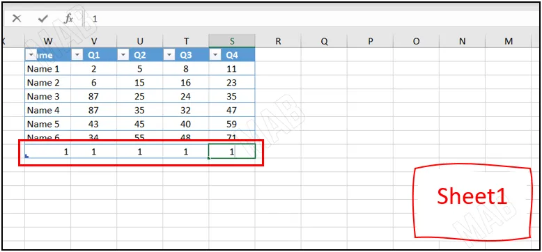
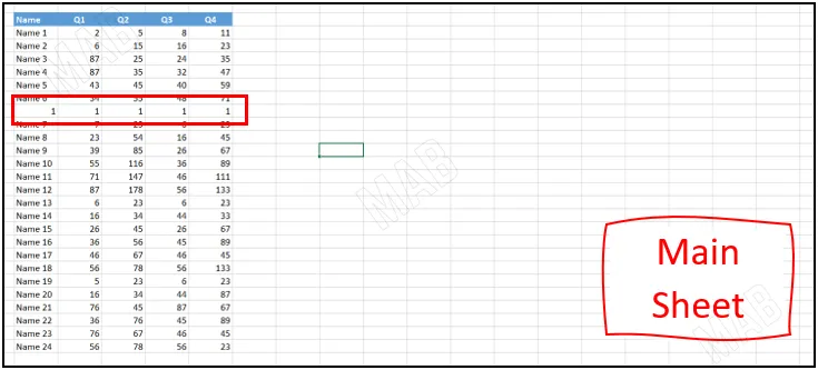
Now when we add any information in any table in one of the sheets (Sheet1, Sheet2, Sheet3, Sheet4), then we press “Enter”, we will notice that the same information is added to the table in the main sheet.
Dear reader, if you liked the article, do not forget to subscribe to our YouTube channel, which provides all new in the field of technical and completely free training courses.
You can also browse our website to access the blog and read technical topics, or learn about the training courses offered by the site.
To access the full course “Excel Course” on YouTube, click here.

