One of the most important features that make us use Excel in particular is the ability to use different types of tables, the most important of which is the pivot table.
Insert a Pivot Table
To use a Pivot Table, it is necessary to first make sure that there are no spaces between the information that we will use. Here is an example of the following information table:
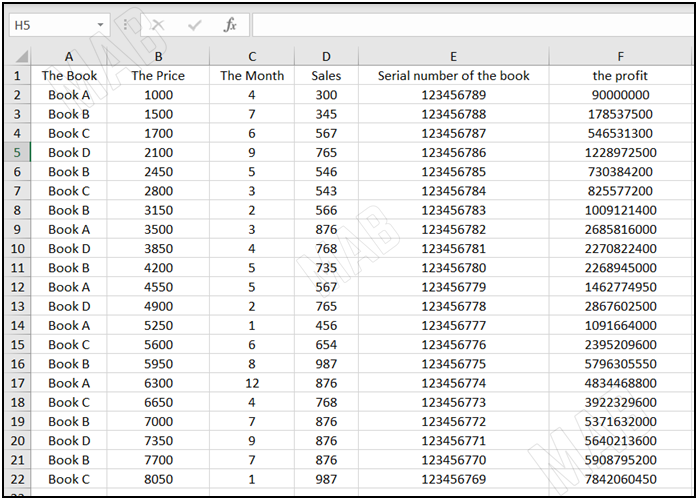
By pressing “Control + A” on any cell within the table, the entire table can be selected to use the Pivot Table.
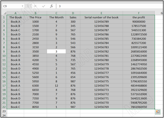
Note: It is preferable to first convert the information into a table so that when we add any new information item, it will be included in the Pivot Table.

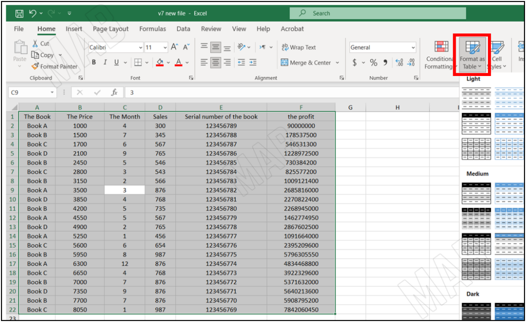
Therefore, we will select the information in the way we mentioned, and through the information bar, we click “Home” and then click “Format As Table”, so the information becomes in the form of a table.
So, after converting the information into a table, we convert this table to a Pivot Table. This is done by going to the information bar clicking “Insert”, and then click Pivot Table.
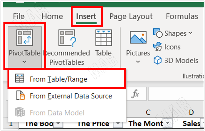
We notice from the options what we talked about previously that when selecting the table, the Pivot Table will include any new information we add to the table, and this is what the first option explains.
As for the second option, we notice the possibility of choosing to work in a new sheet or in the same sheet, and here we will choose to work in a new sheet to clarify the work.
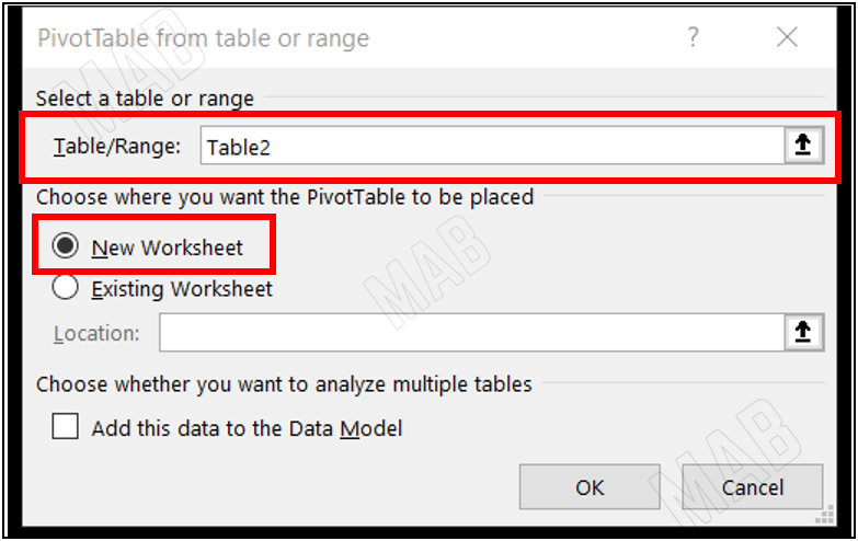
Now a new worksheet will open and the Pivot Table will be in it, and we will notice on the right side of the sheet the group of elements that make up the Pivot Table:
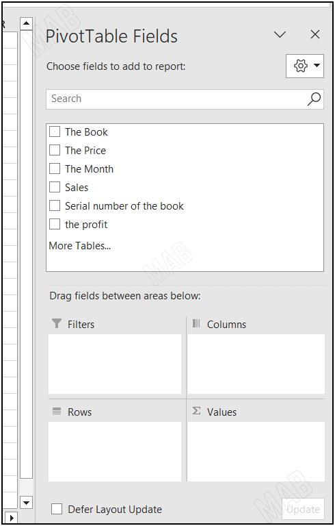
We will also notice that there are four options:
- Columns to choose the elements that will be tables.
- Row to choose the elements that will be rows.
- Values to choose the elements that will be values.
- Filter to make one of the elements a filter.
Different ways to arrange information
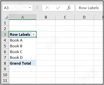
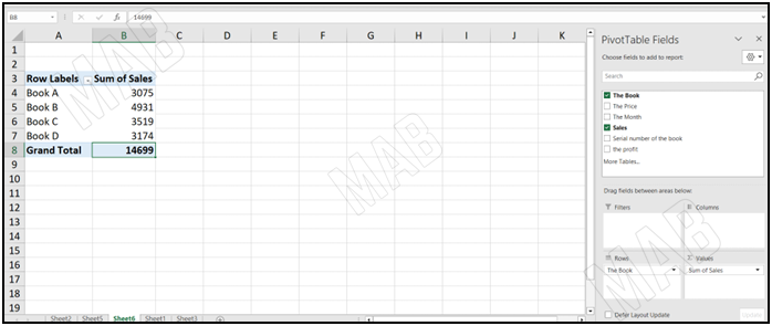
Now we put the “book” within the “rows” by dragging and dropping, and we notice that the books appear as separate rows.
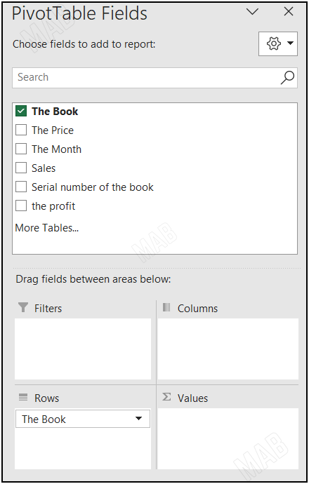
We notice that the names of the books are many, but in the end, they are the names of four books. Thus, the Pivot Table summarizes them into four books, as we notice in the picture.
We can also put “sales” in the values, so they appear as follows:
We can also add “month” to “books” in the rows.
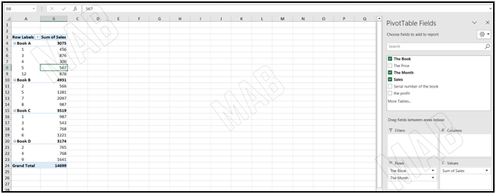
We notice how the book appeared and the month below it, where the order is important here, so if we want the month to appear and the book below it, we reverse the order.
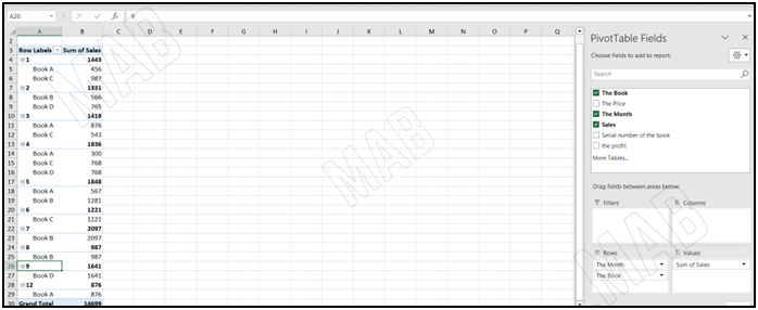
We notice that the Pivot Table collects information in a very smart way. We notice that when we add each of the books, months, and the number of sales, it collects the number of sales for each month from the point of view of each book.
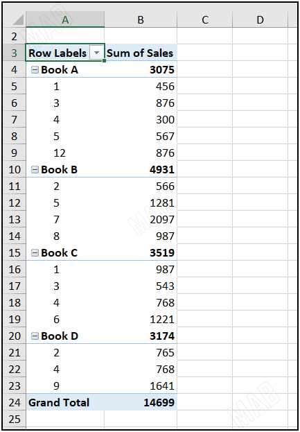
As for book B, the number of sales for the fifth month was 1281, and the total sales were 4931.
We can also add the month to the “Columns”, and thus we get the following form:
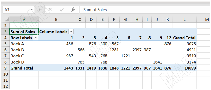
Grand Total box
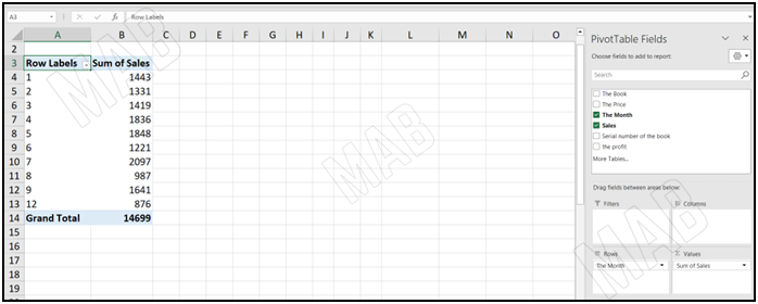
Let us say we want to see the entire month’s sales without the names of the books, so we put “Sales Number” in “Values” and “Month” in “Rows”.
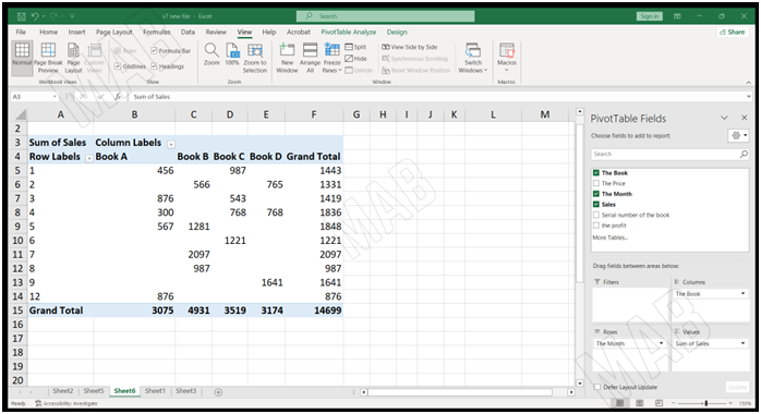
Now if we put “Month” in “Rows”. And put “Book” in “Columns”. Then put “Sales” in “Values”. We finally notice the appearance of the “Grand Total” box that shows the total sum of the values.
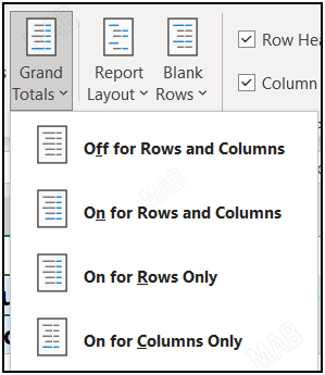
If we want to remove this box, we go to the toolbar and then to “Design”. After that, we choose “Grand Total”, click “Grand Total” and then click “Off for Rows and Columns”.
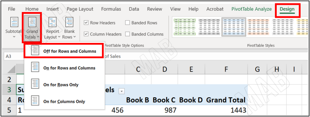
We notice from the options that I can:
– First, show the total for columns only “On for Columns Only”
– Then show the total for rows only “for Rows Only On”
– After that, show the total for columns and rows “On for Rows and Columns”
– And finally, hide the total completely “for Rows and Columns Off”.
Using the Filter feature in the pivot table
To use the “Filter” feature, we put the month in “Rows”, the number of sales in “Values”, and the book in “Filters”.
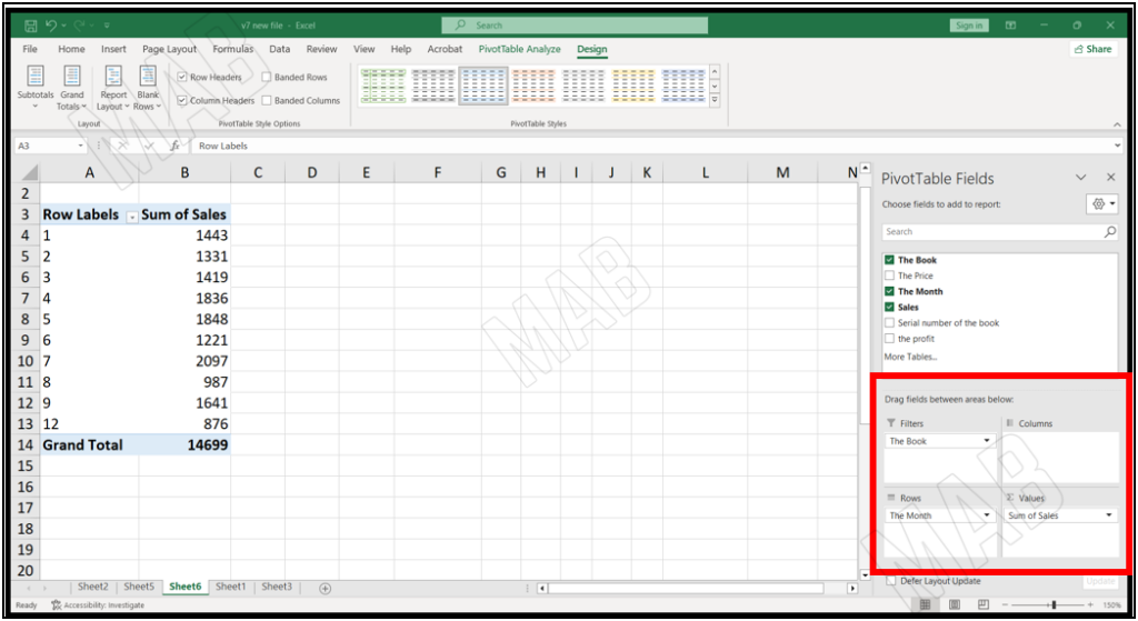
Thus, we notice that it has become possible to choose between several books using the arrow.
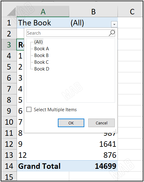
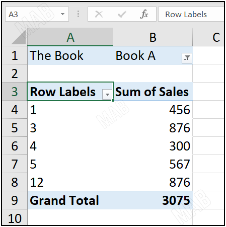
We choose one of the books and then click Ok, so we can see the number of sales for this book each month.
We can also select more than one item from the “Filters”, through the option “Select Multiple Items” and then select more than one item.
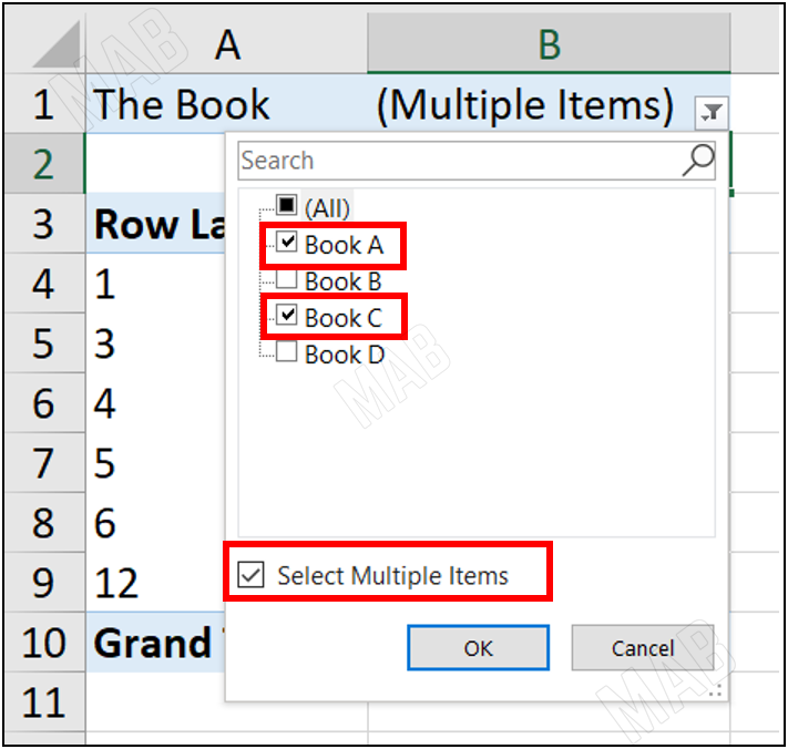
In this case, the result will be to add the sales of the two books and put them in the number of sales box.
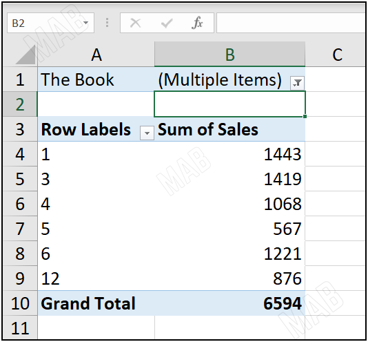
Note: If we want each book to appear separately, we must put the book within the “Rows” or “Columns”. We can also change the shape of the table from the toolbar by choosing “Design”, and then choosing from the available designs for the table at the top.

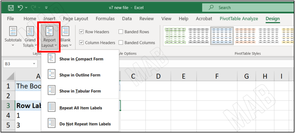
We can also get other options for the table style through the “Report Layout” options.
Dear reader, if you liked the article, do not forget to subscribe to our YouTube channel, which provides all new in the field of technical and completely free training courses.
You can also browse our website to access the blog and read technical topics, or learn about the training courses offered by the site.
To access the full course “Excel Course” on YouTube, click here.


