In this lesson, we will learn how to organize information in Excel in seven different ways.
First, in order to clarify the idea, we will create a set of data in Excel, which are names in English.
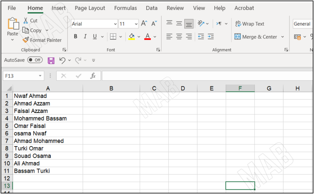
How to make all letters uppercase in Excel – Organize information in uppercase
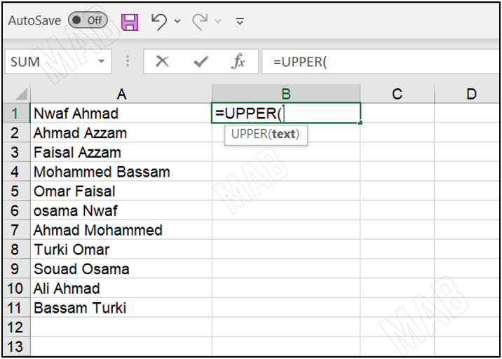
After writing the data set, we go to the corresponding cell and type “upper=” and the upper shortcut appears. We click on it and it asks us to enter text (text).
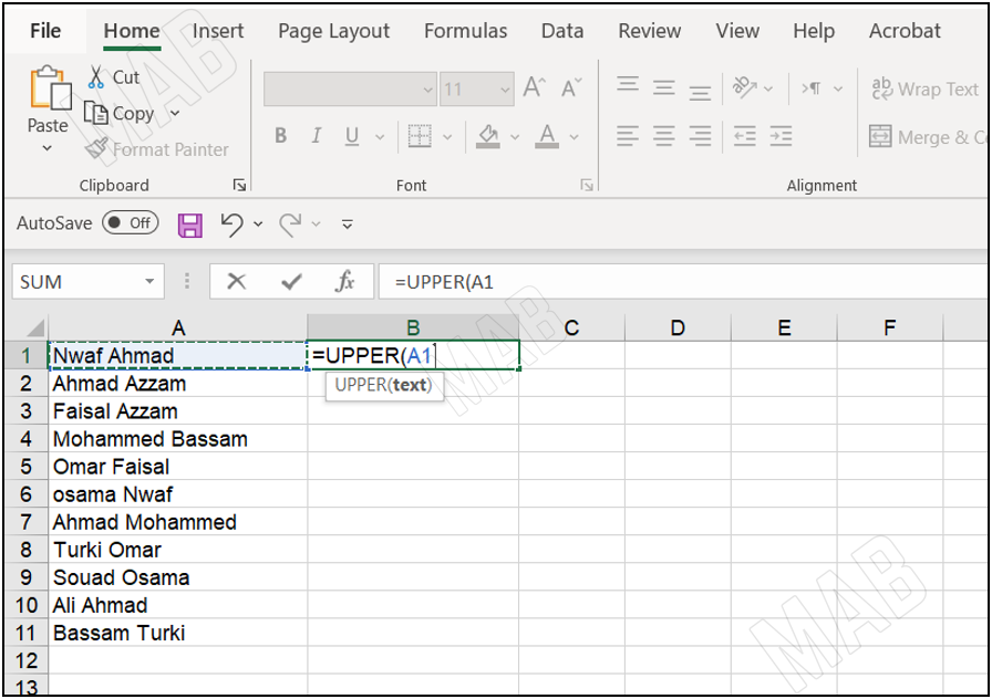
We now select the cell in which we will capitalize the letters of the names.
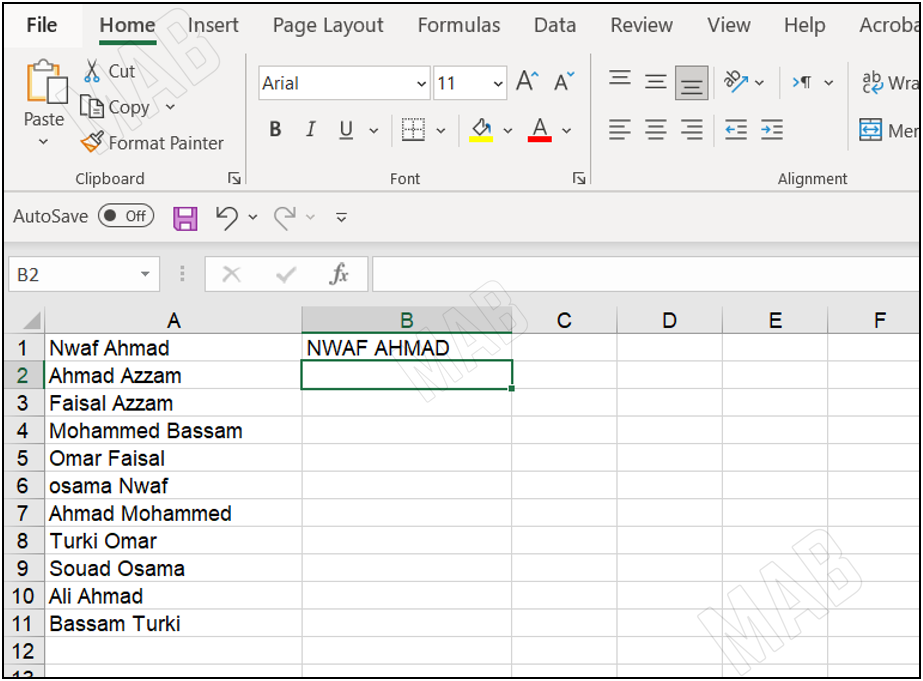
Then we press “Enter” and notice that all the word’s letters have become uppercase.
To format all the information in the same way, we will drag down starting from the resulting cell and in the same direction as the remaining cells as follows:
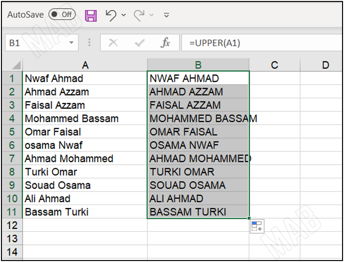
Then we release the mouse and notice that all the information has become uppercase
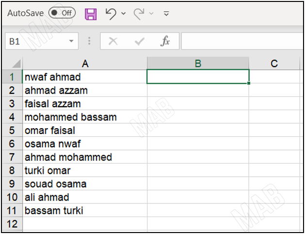
Organize information in lowercase letters in Excel
After writing the data set, we move to the corresponding cell and type “lower=”
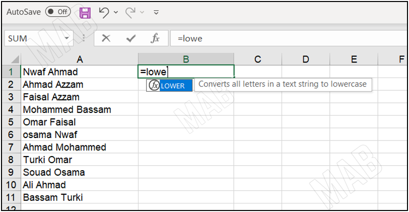
Then the shortcut lower appears and we click on it and it asks us to enter text (text).
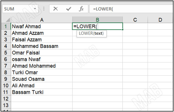
After that, we now select the cell in which we will make the letters of the information contained in it small.
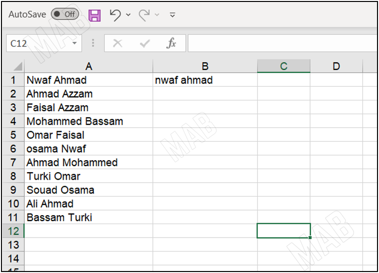
Then we press “Enter” and notice that all the word’s letters have become small.
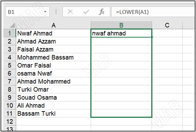
As for arranging all the information in the same way, we drag down starting from the resulting cell and in the same direction as the remaining cells as follows:
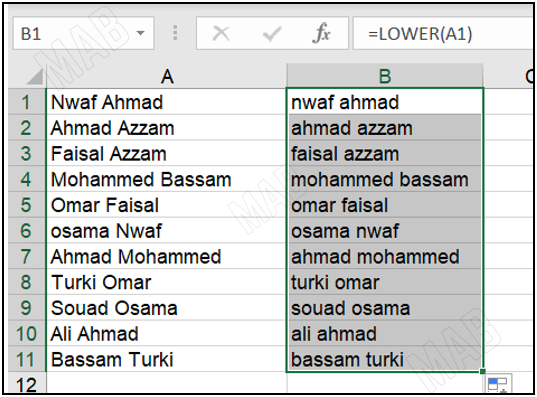
Then we release the mouse and notice that all the information has become small letters.
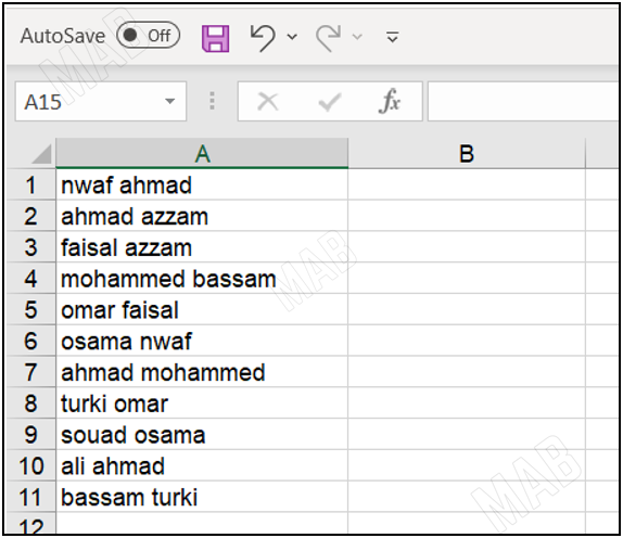
Organize information by making the first letter capitalized in Excel
Let us have the following information, all written in lowercase.
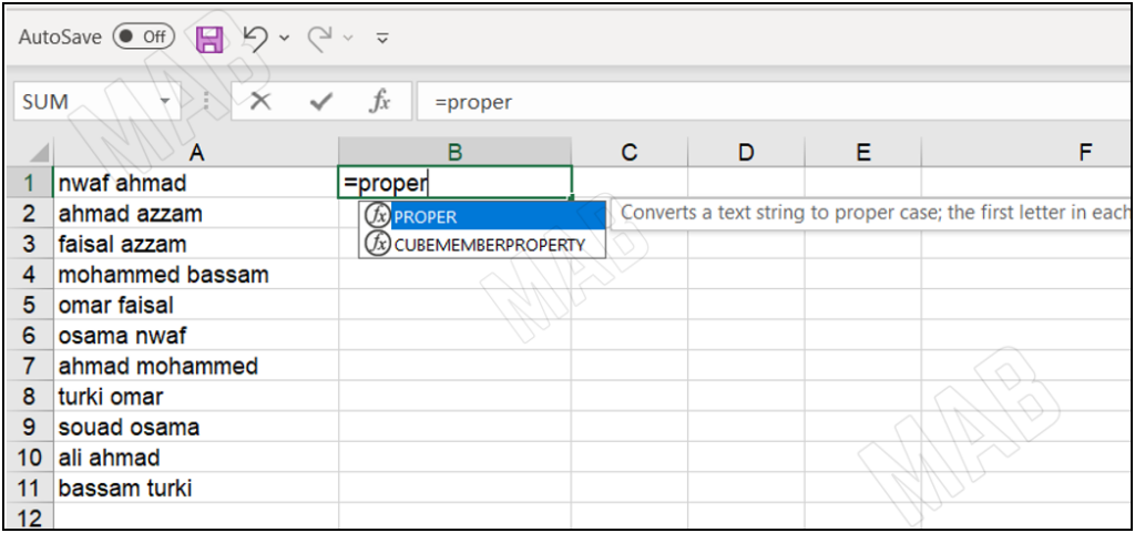
After writing the data set, we move to the corresponding cell and type “Proper=”, and then the shortcut “PROPER” appears. After that, we click on it and it asks us to enter text (text).
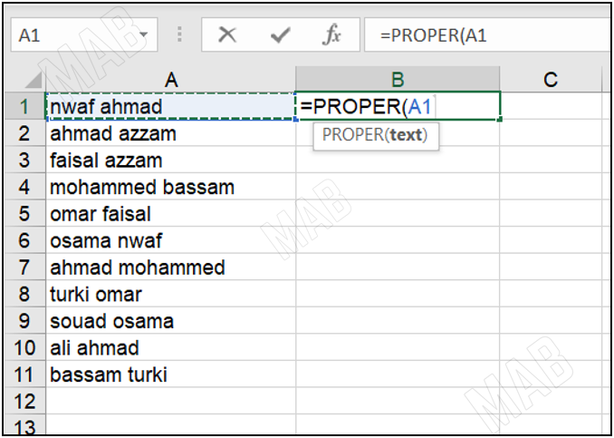
We now select the cell in which we will make the first letter of the information contained in it capitalized.
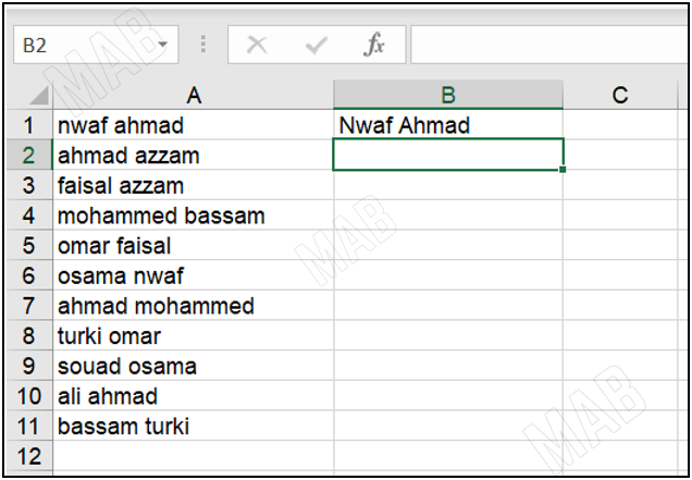
Then we press “Enter” and notice that all the first letters of the word have become capitalized.
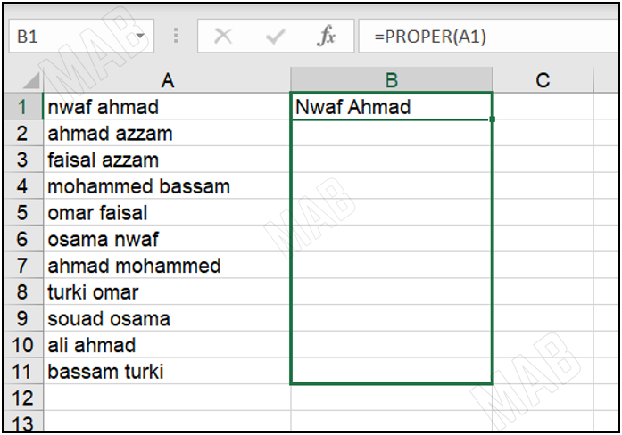
To format all the information in the same way, we drag down starting from the resulting cell and in the same direction as the remaining cells as follows:
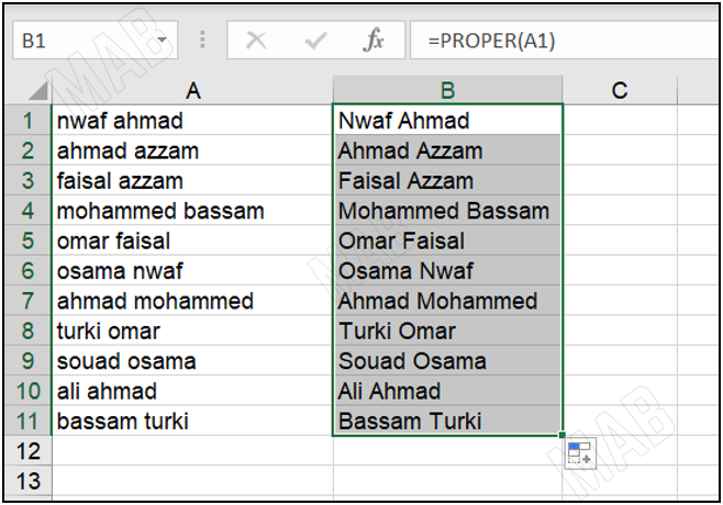
We release the mouse and we notice that all the first letters of the word have become capitalized.
How to combine two cells into one cell in Excel – Organize the information of two or more cells into one cell
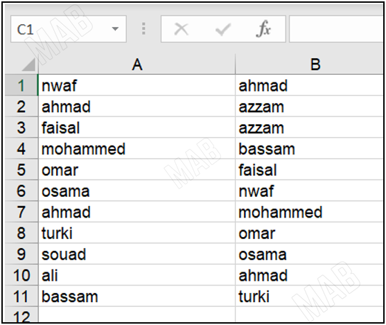
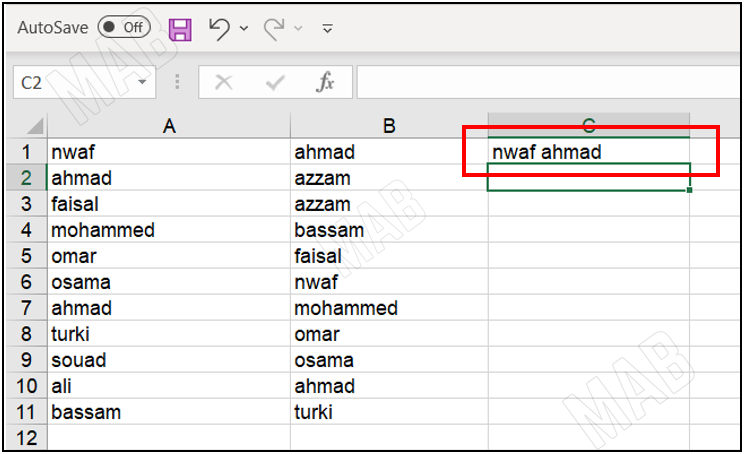
Let us have two columns of data, the first column forms the first name, and the second column forms the last name and we want to combine them to form a full name.

We have two ways to combine two cells into one cell:
The first method:
First, we put the “=” sign inside the cell in which we want to put the information for the two cells.
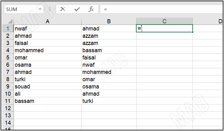
Then we write the name of the function for the operation, which is “Concat”, and the function shortcut appears, so we select it.
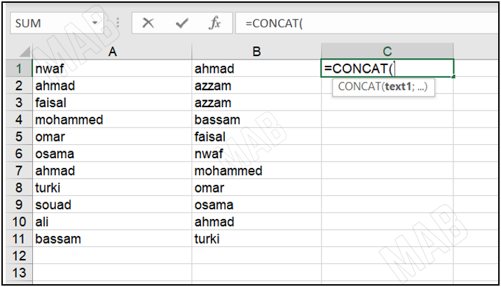
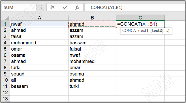
When selecting the function, we will be asked to enter text (Text), and here we select the two cells whose contents we will combine into one cell.
But we will distinguish the following two cases:
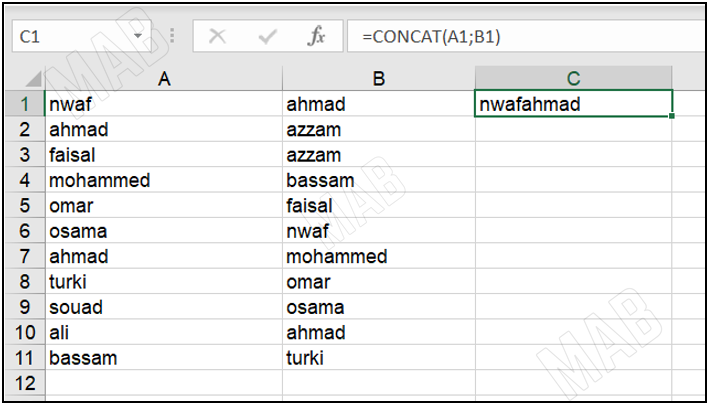
- If we select the two cells whose contents we will combine and there is a comma between them and we press “Ok”, then the contents of the two cells will appear adjacent with no space between them.
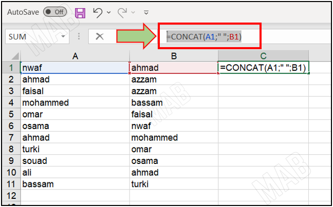
- To put the contents of the two cells in one cell with a space between them, we add a space as follows: =CONCAT(A1;” “;B1)
Then this space is added at the top under the toolbar in the place where the function is written.
We can also add spaces between the quotation marks as much as we want to appear between the contents.
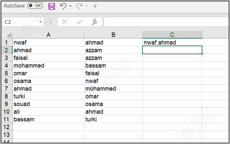
Then we press “Enter” and the contents of the two cells appear inside the common cell with a space between them.
The second method:
First, we put the “=” sign inside the cell in which we want to put the information about the two cells.
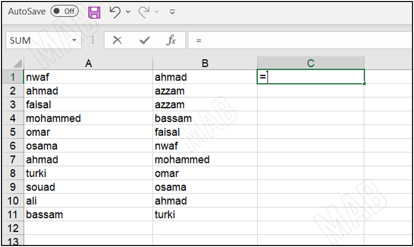
We choose the first cell that we want to combine and then we use the “&” sign and then select the second cell.
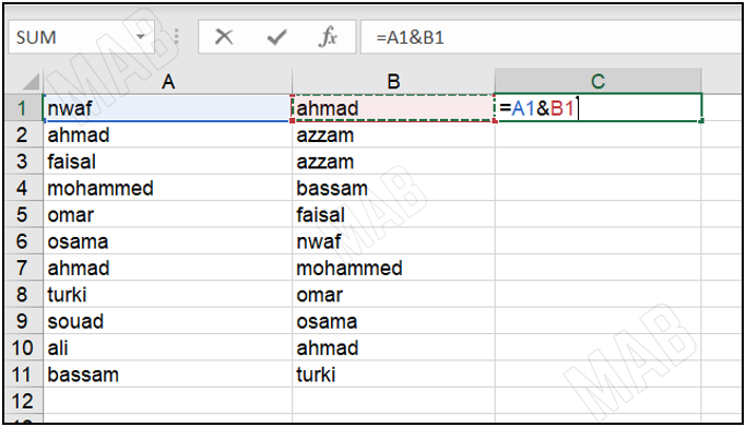
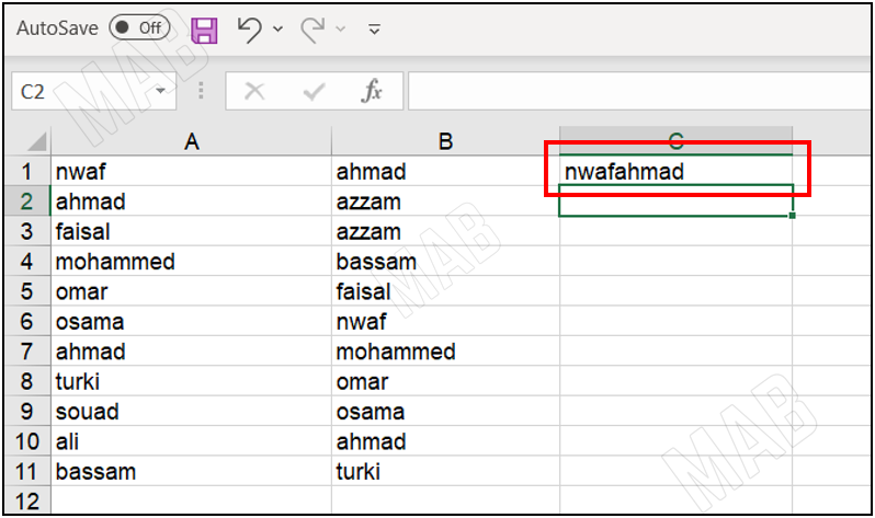
Then we press “Enter” and the contents of the two cells appear inside the new cell.
If we want to add spaces, we do so using the “&” sign as follows:
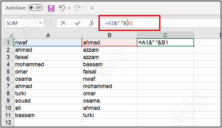
Then we press “Enter” and the contents of the two selected cells appear with spaces between them in the number of spaces we added after the “&” sign between the quotation marks.
How to remove spaces between information inside cells in Excel – Organize information and remove extra spaces
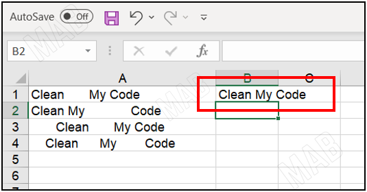
To clarify the idea, we will use a set of data that contains many spaces.
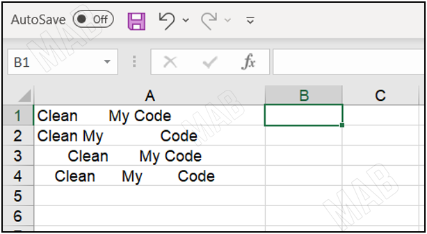
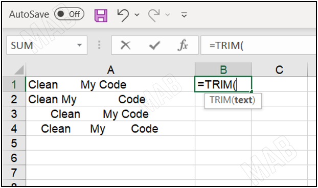
To remove the spaces that appear between words, we will use the “Trim” function, where we put the “=” sign in a new cell and then write the “Trim” function.
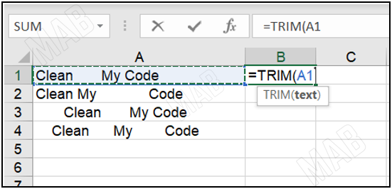
The function asks us to enter text, so we select the cell in which we want to remove the spaces between the words.
Then we press “Enter” and notice that the extra spaces between the words have been removed.
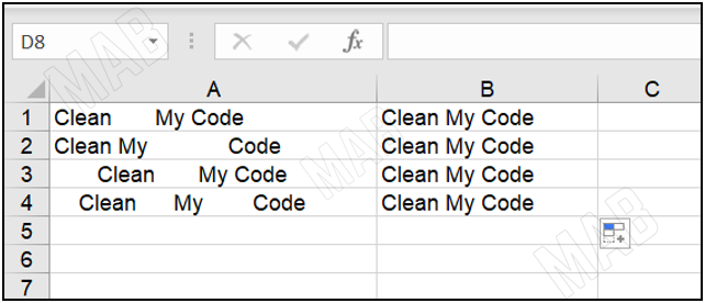
By dragging the new cell downward, we will notice that the process has been applied to all cells.
How to know the length of information inside cells in Excel
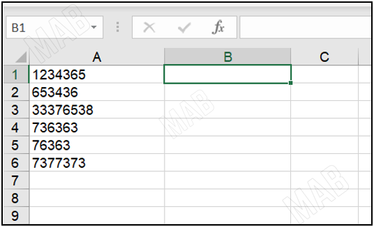
To clarify the process, we will prepare a group of cells that contain data in the form of numbers of different lengths.
To know the length of each number, we will use the “Len” function.
So first, we will write the “=” sign in a new cell and we will write the Len function.
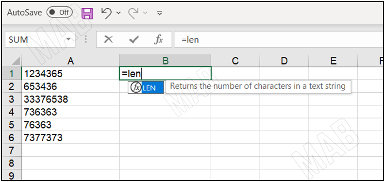
Then after selecting the “Len” function, we will be asked to enter text and select the cell in which we want to know the length of the information contained.
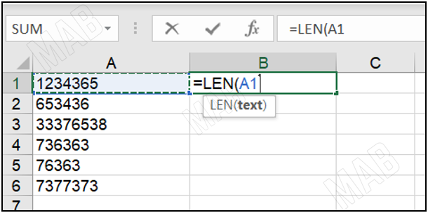
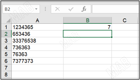
Then we press “Enter” and we will notice that the result is the number of numbers in that cell.
By dragging the new cell downwards, we will apply the process to all cells.
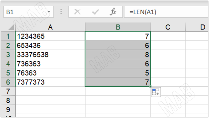
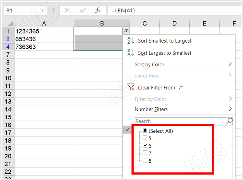
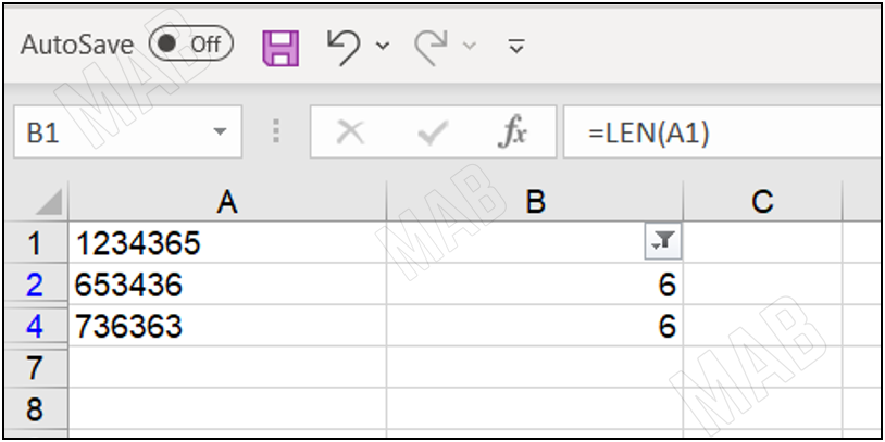
If one of these data is the required data, for example, if the required length of the information is 6 and we want to select only the information whose length is 6, in this case, the “Filter” feature can be used.
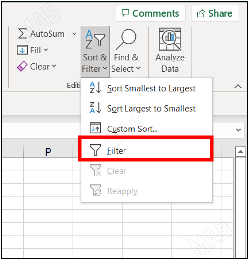
The “Filter” feature can be obtained from the “Sort & Filter” toolbar after we select all the resulting data.
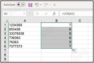
Then we click on the “Filter” option.
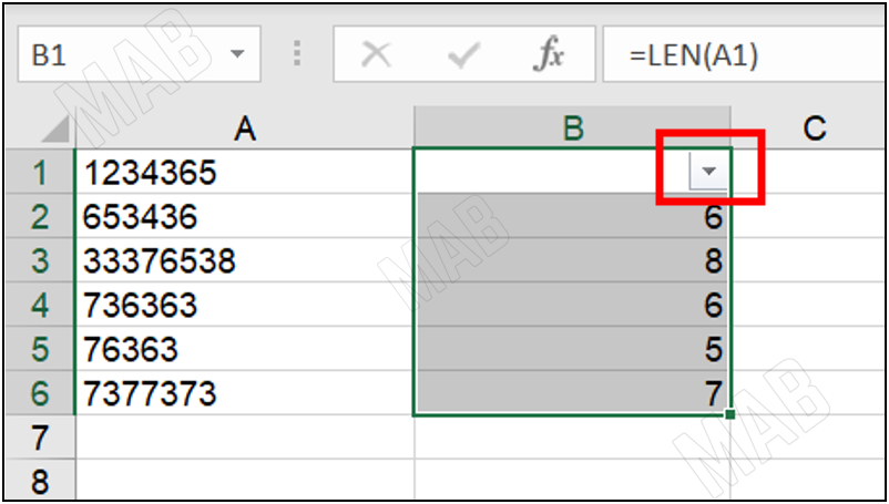
We will notice a small arrow mark next to the table of lengths of the information that we have selected.
We click on the arrow and an interface appears through which we can choose the number 6 to display only data with a length of 6.
How to remove duplicates in Excel
To clarify the idea, we will prepare the following table that contains two duplicate names with their data.
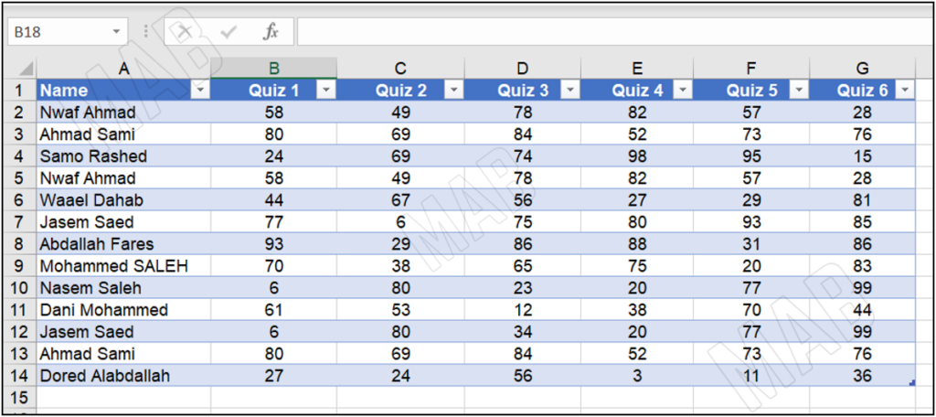
Duplicate detection
- First, we select the entire table by: “control” + “A”.
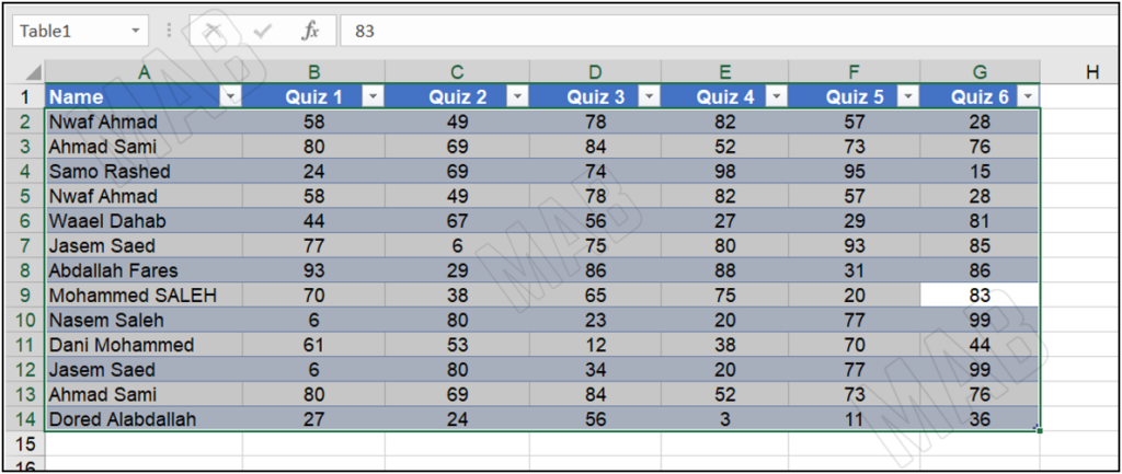
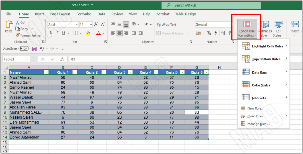
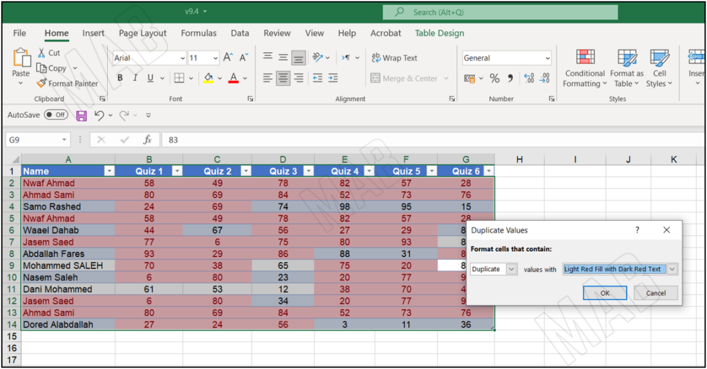
- Second, from the toolbar and then from “Table Design” we choose “Conditional Formatting”.
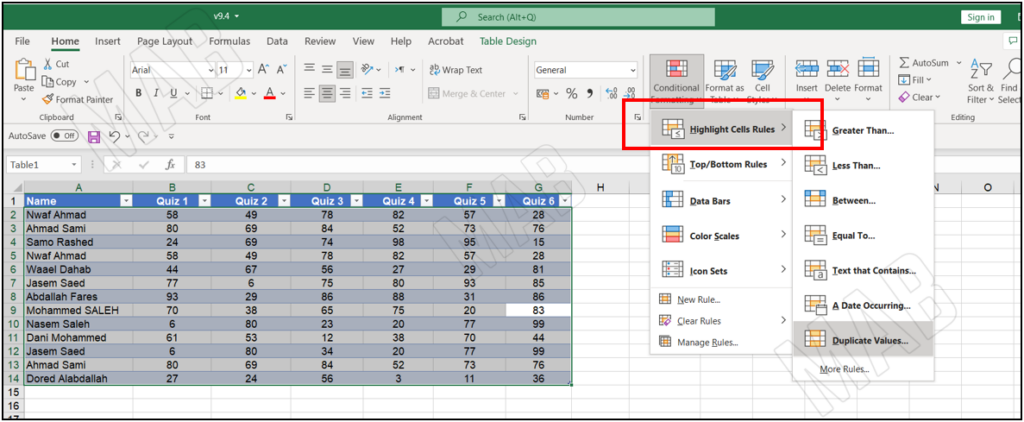
- Then from “Highlight Cells Rules” we choose “Duplicate Values”.
- After that, we notice from the interface that it appears that we want to select the duplicate values and that we can specify the color of the duplicate values (here we will leave them in red) and then click “Ok”.
We notice how the duplicate values appeared in red.
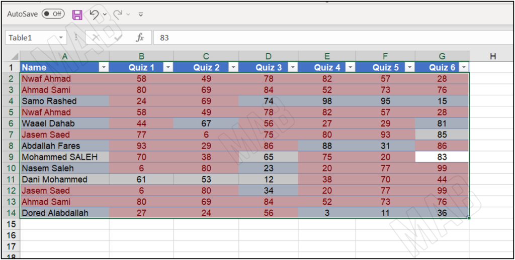
Note:
You can know that the duplicate is complete (the name is repeated with the marks and therefore the entire information is duplicated) through the red color on an entire line.
Removing duplicates from information
- First, we select the entire table using “Control + A”.
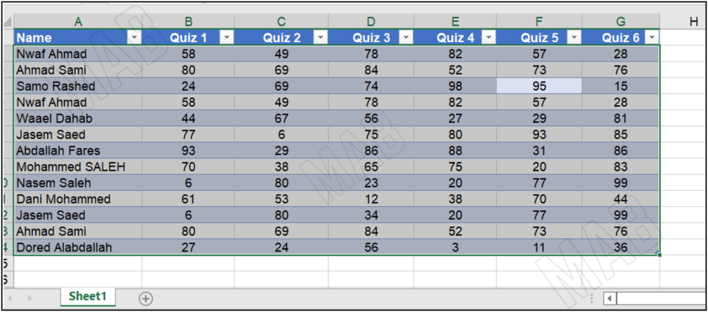
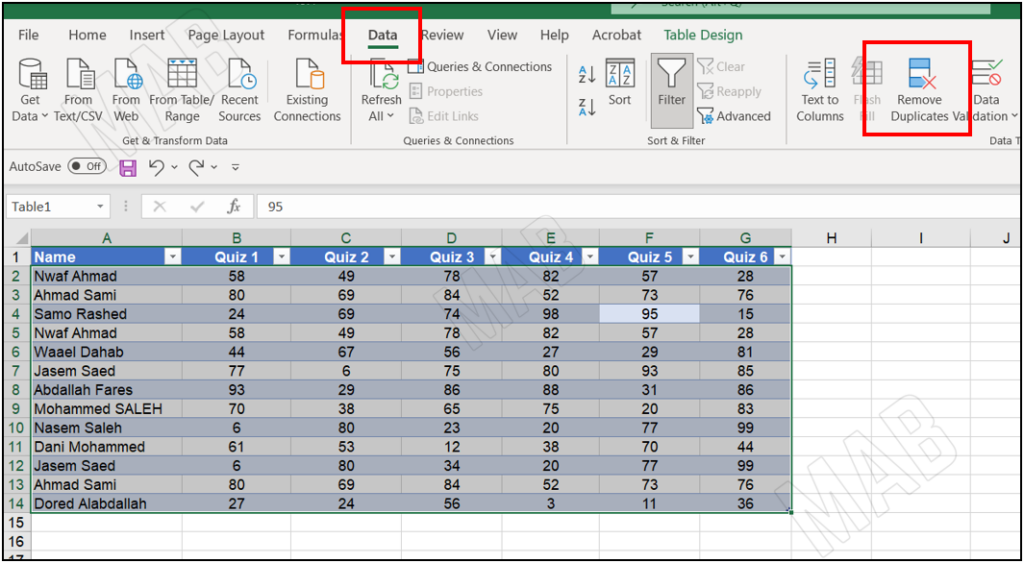
- Second, from the toolbar, we choose “Data” and then choose “Remove Duplicates”.
- Then an interface appears from which we select all the existing elements that represent the table titles in order to delete only the complete duplicate.
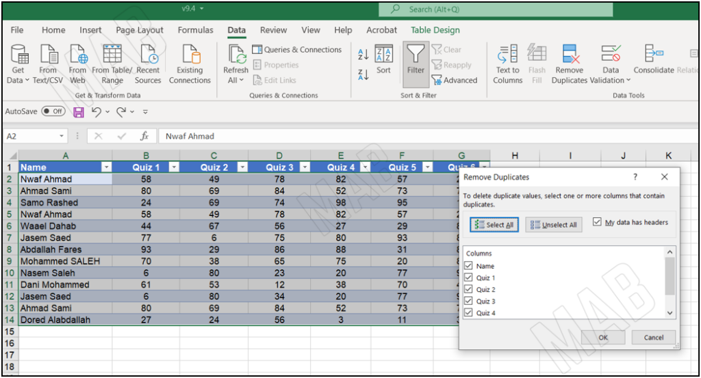
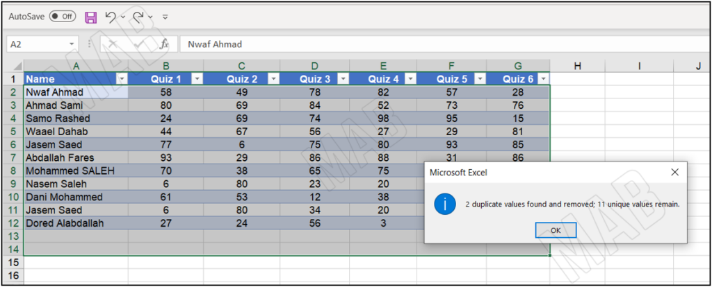
- Then we click “Ok” and we notice that the duplicate information has been completely removed.
Dear reader, if you liked the article, do not forget to subscribe to our YouTube channel, which provides all new in the field of technical and completely free training courses.
You can also browse our website to access the blog and read technical topics, or learn about the training courses offered by the site.
To access the full course “Excel Course” on YouTube, click here.


