In this lesson, we will learn how to filter information and get similar information in the easiest way using the slicer tool in Excel.
If we have a large amount of information as follows:
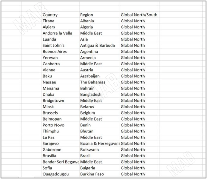
We will need a way that enables the user to filter the information in a visual and easy way.
Create a table from the available information
First, click on any cell in the information, and from the keyboard, choose “CTRL + A” to select all the information.
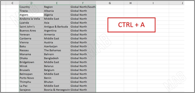
Also from the keyboard, press “CTRL + T” to convert the information to a table, then choose “Ok”.
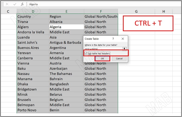
Note: Do not forget to select the option “My table has headers” to make the first cell in each column the title of the column.
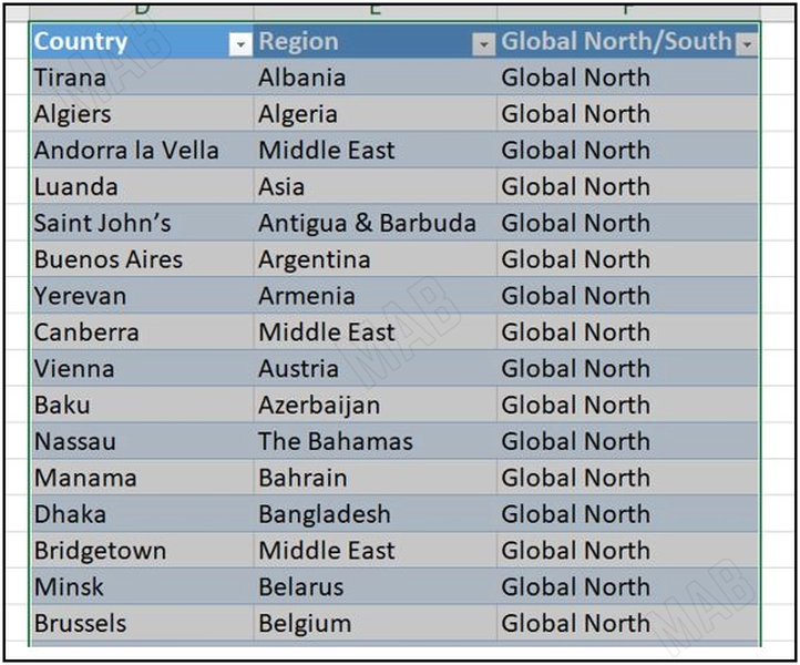
As a result, we have an Excel table containing the information as follows:
Create a slicer filter tool
The next step is to go to the toolbar, then choose “Table Design”, and we will find the option “Insert Slicer” to use the filter tool.

If we now choose “Region” for example, the information will be filtered according to “Region”.
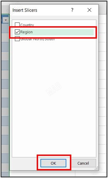
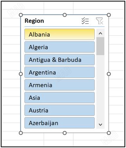
We click “Ok” to see the result, and an interface will appear with many buttons used for filtering, this interface is called “Slicer”.
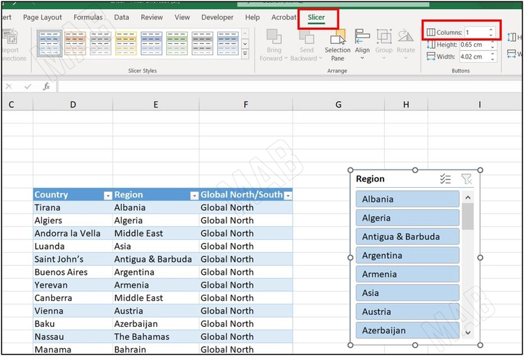
If we want the “Slicer” to appear at the top of the table, and for example to become a group of columns instead of one column. Therefore, I will click on the “Slicer” option from the toolbar.
From the “Columns” option, we can increase the number of columns to four for example, so we will get this shape.
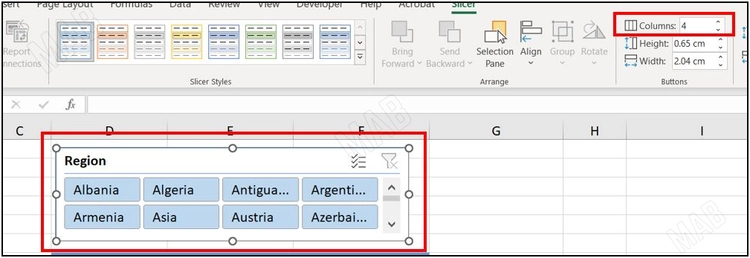
Now we can use it by clicking on the slicer buttons.
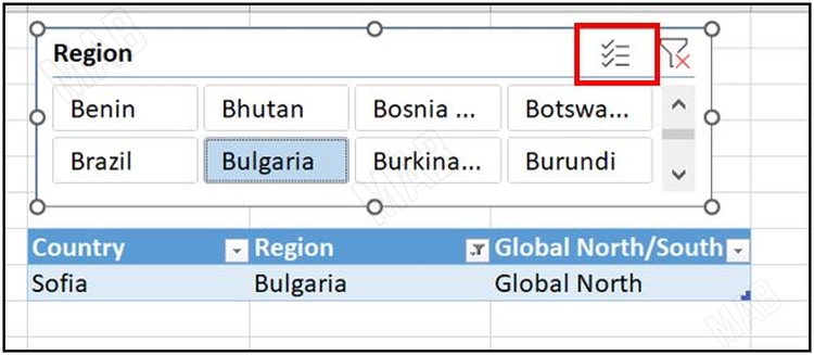
We can also use the sign at the top of the “Slicer” to select more than one option.
Dear reader, if you liked the article, do not forget to subscribe to our YouTube channel, which provides all new in the field of technical and completely free training courses.
You can also browse our website to access the blog and read technical topics, or learn about the training courses offered by the site.
To access the full course “Excel Course” on YouTube, click here.

