In this lesson, we will learn how to use a Dropdown List in Excel.
Assuming we have a set of options, these options express sizes, which are (S, M, L, XL, XS).
In return, we have a set of names that we will follow these sizes.
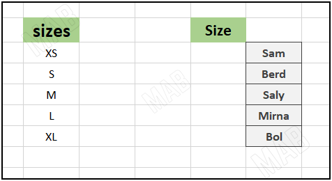
It is useless in this case to write the name of the size for each person’s name, especially if the information is large.
The solution is to use the dropdown list according to the following steps:
1- We select the list for sizes.
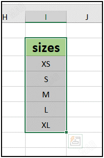
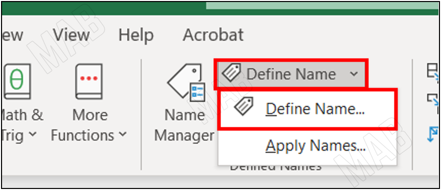
2- From the toolbar and from “Formulas” we choose “Define Name”, and leave the name as is or change it as desired.
But in this example, we will leave the name “Sizes”.
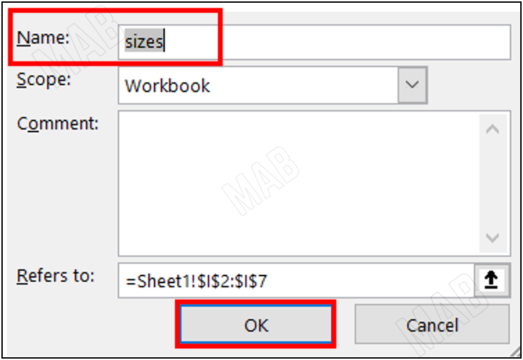
3- We click “Ok” and then we select the column in which we will use the list.
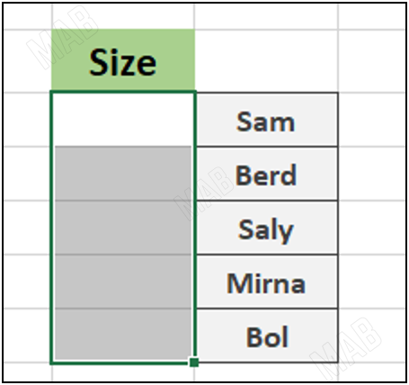
4- From the toolbar and from “Data” we choose “Data Validation”.

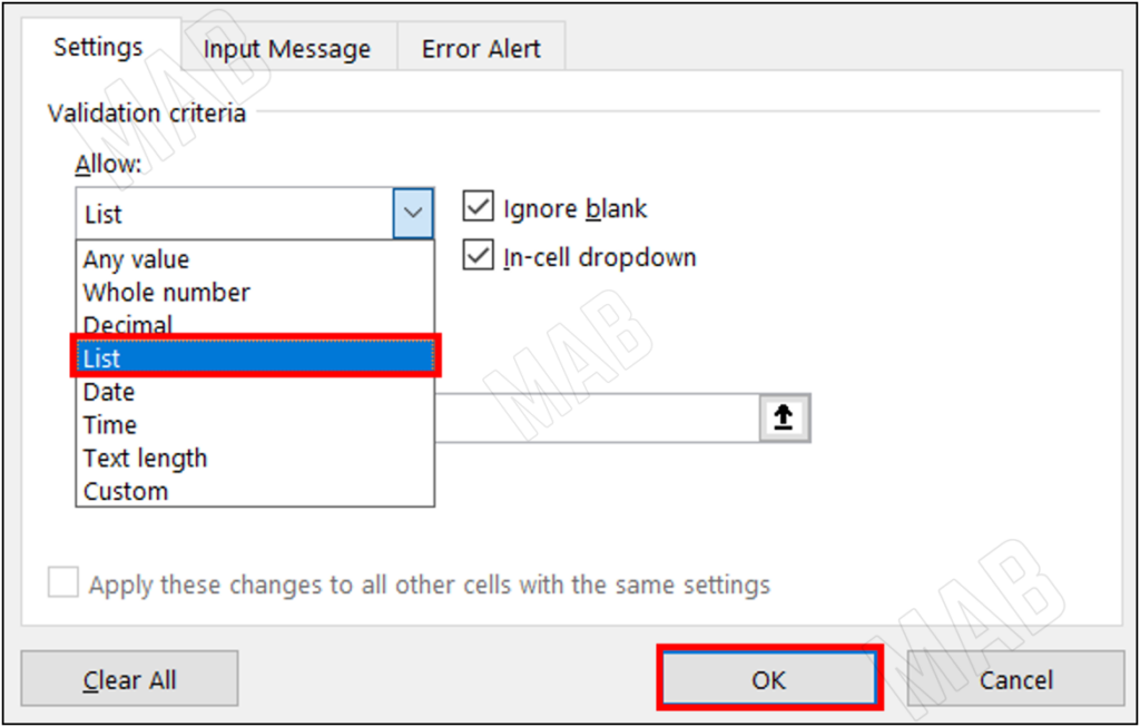
5- From “Data Validation” we will choose the elements that we will use within this specific column, which are the sizes here, so we will choose the option “List”.
6- Then we will select the list of sizes.
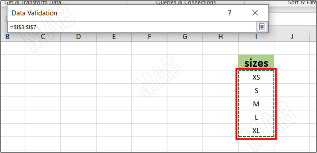
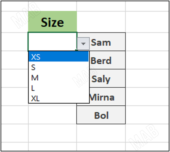
7- Press “Enter” and then choose “Ok”. Here we notice that the sizes are now available for each name.
Dear reader, if you liked the article, do not forget to subscribe to our YouTube channel, which provides all new in the field of technical and completely free training courses.
You can also browse our website to access the blog and read technical topics, or learn about the training courses offered by the site.
To access the full course “Excel Course” on YouTube, click here.


