In this lesson, we will learn comparing percentages using conditional formatting in Excel.
Suppose I have the following information table.
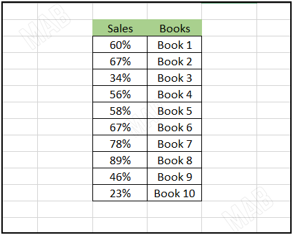
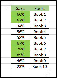
And I want to choose from it the percentage of 60% or more and distinguish it with a different color.
Define the percentages that are equal to or greater than 60% in green
We will do the following steps:
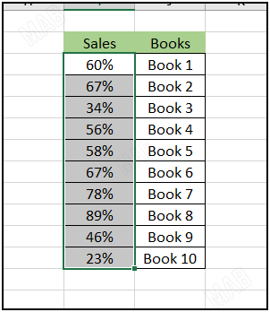
1- We select all the percentages cells.
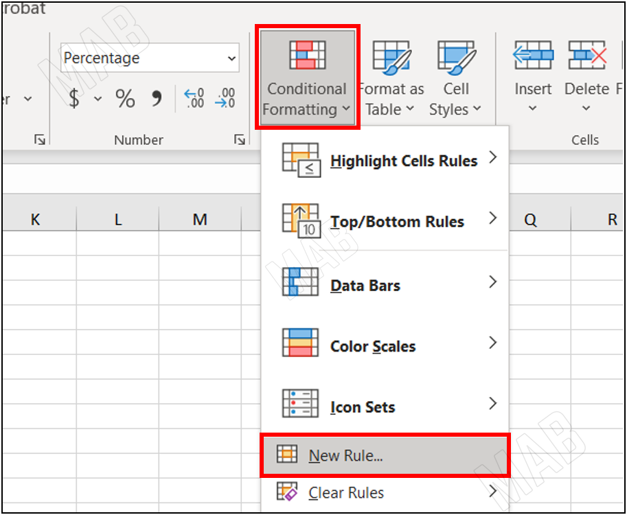
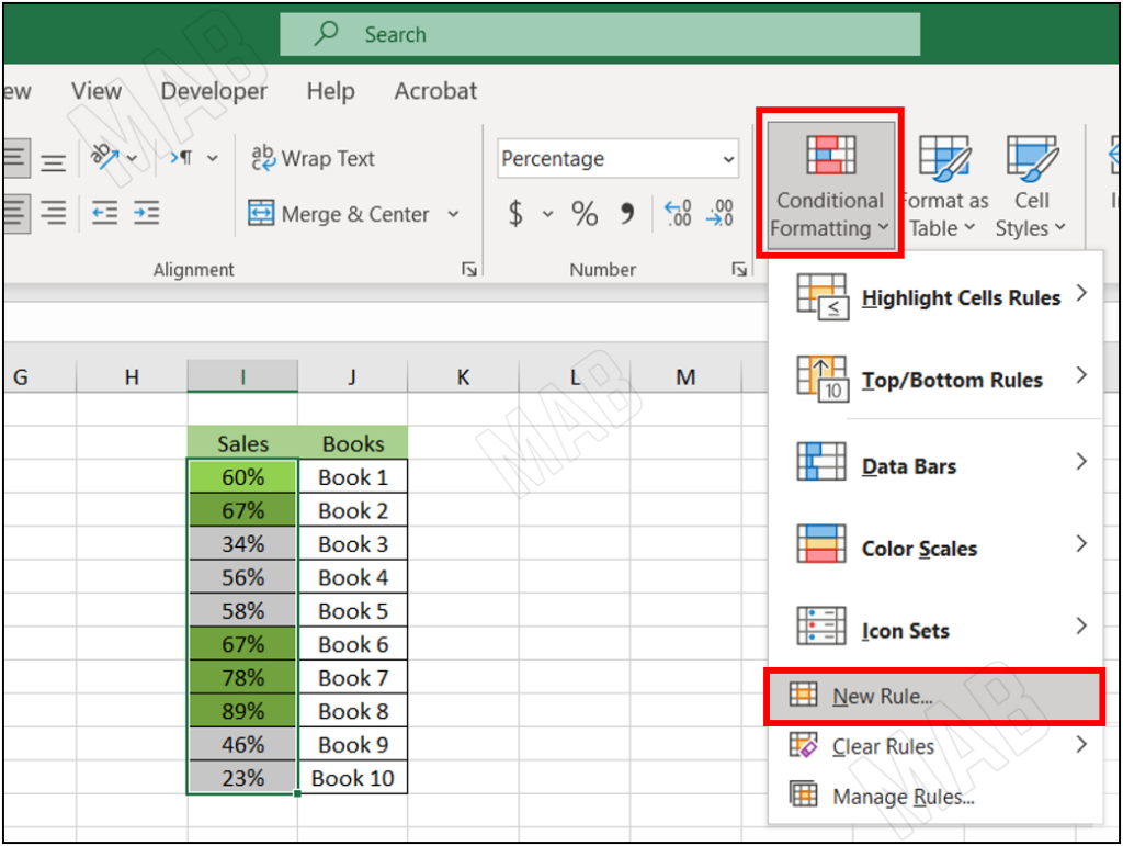
2- From “Conditional Formatting” we choose “New Rule”.
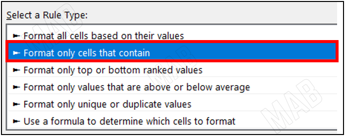
3- From it we will choose the second option.
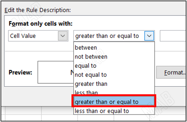
4- From “Format only cells with” and from “between” we will choose “Greater than or equal to”.
In the blank we will put 60%.
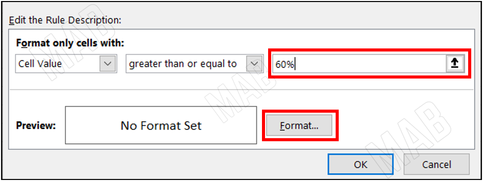
5- After that, from “Format” we will choose the color with which we will distinguish the cells.
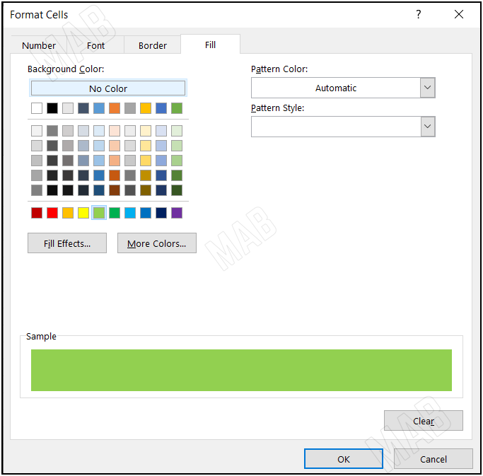
6- Finally, we choose ok.
Define the percentages less than 60% in red
To define the percentages less than 60% in red we repeat the same steps as follows:
1- First, we select all the percentages.
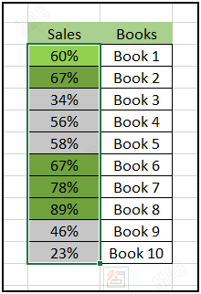
2- Then, from “Conditional Formatting” we choose “New Rule”.
3- From it we will choose the second option.

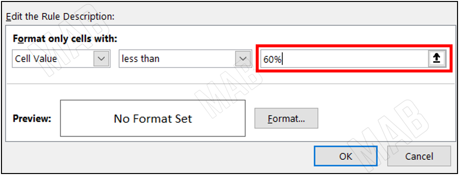
4- From “Format only cells with” and from “between” we will choose “less than”.

In the blank, we will put 60%.
5- Then, from “Format” we will choose the color we will use to distinguish the cells.
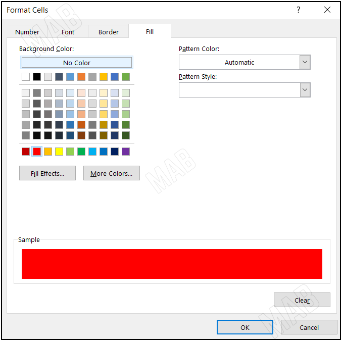
6- After that we choose ok.
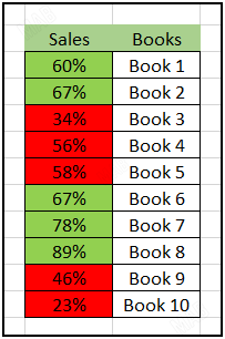
excel-conditional-formatting-percentages
Dear reader, if you liked the article, do not forget to subscribe to our YouTube channel, which provides all new in the field of technical and completely free training courses.
You can also browse our website to access the blog and read technical topics, or learn about the training courses offered by the site.
To access the full course “Excel Course” on YouTube, click here.


