In this lesson, we will learn How to select empty cells in Excel using conditional formatting.
Let’s start by assuming we have the following table:

In order to remove empty cells, we will follow the following steps:
1- We select the entire table.

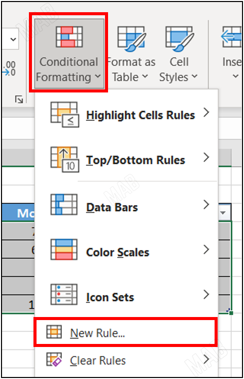
From the toolbar, from “Home” we choose “Conditional Formatting”, from which we will choose “New Rule”.

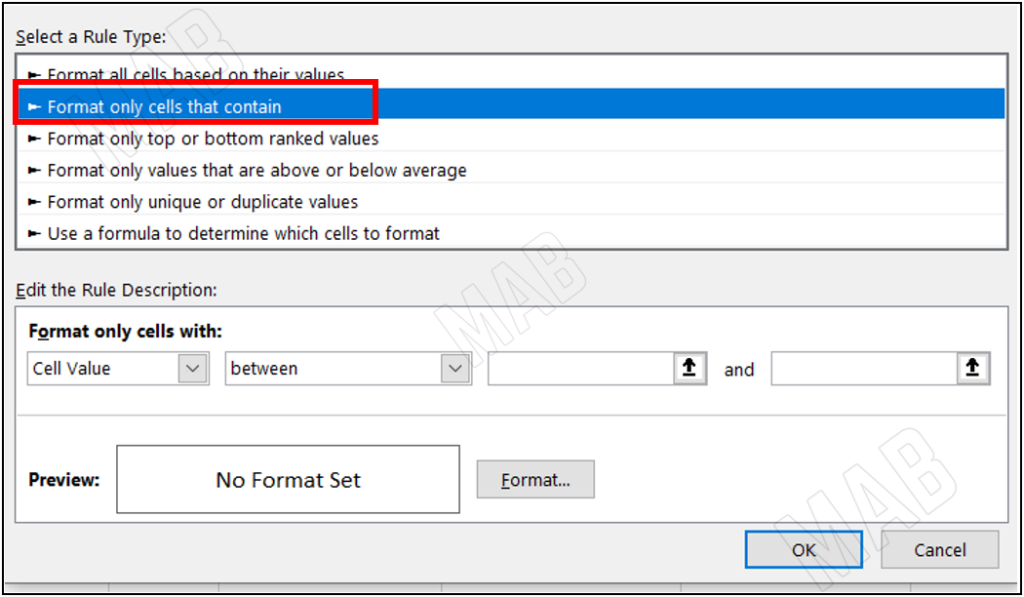
The following interface will appear, from which we will choose the second option “Format Only Cells That Contains”.

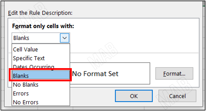
From the bottom, we will choose the cells that contain blanks “Blanks”.

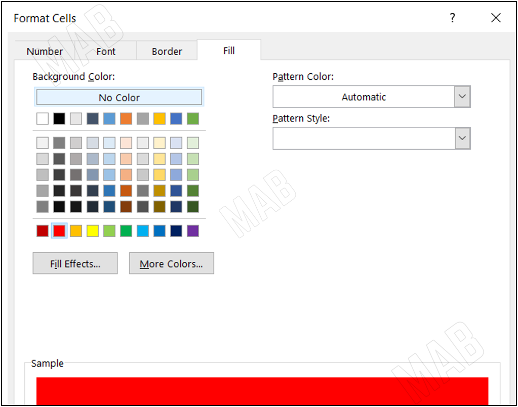
From “Format”, we will determine how the format of the empty cells will look, and in this example, we will make the empty cells red.

We choose “Ok” and the result will be as follows.

We notice that when adding any expression to an empty red cell, the red color disappears.

Dear reader, if you liked the article, do not forget to subscribe to our YouTube channel, which provides all new in the field of technical and completely free training courses.
You can also browse our website to access the blog and read technical topics, or learn about the training courses offered by the site.
To access the full course “Excel Course” on YouTube, click here.


