In this lesson, we will discuss the topic of charts in Excel and all the processes related to them, with a full explanation using live examples.
In this lesson, we will learn how to name cells in Excel using the Name Manager option to use them in other future operations that we will learn about in the upcoming lessons.
Manually changing the cell name in Excel
First, to change the name of any cell in Excel, we can simply do the following steps:
• First, we select the cell we want to name.
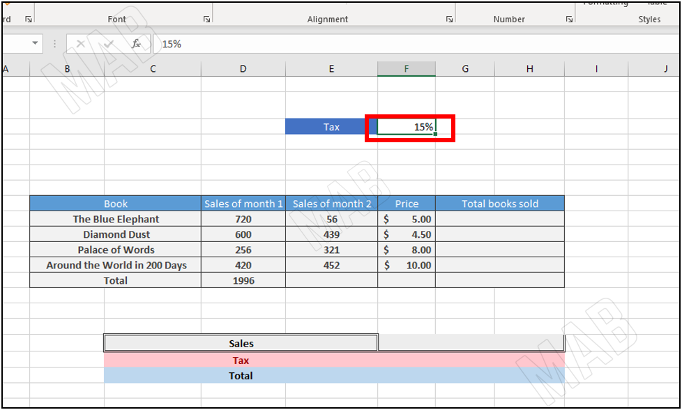
• Then we notice at the top a small box through which we can change the cell name.
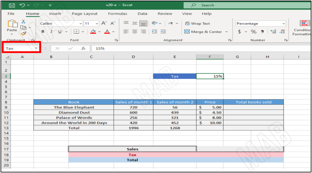
Note: It is necessary that the names are without spaces and that the name is complete so that errors do not occur.
But if we want to use this cell for “Formulas” purposes, this method is not useful and it will be necessary to use the Name Manager feature.
Using the Name Manager feature
To sum the sales of the first book in month 1 and the sales of the first book in month 2.
Assuming we want to keep a name for this sum to use it elsewhere at another time, we will do the following steps:
• First, we select the two cells to which we want to apply the summation process.
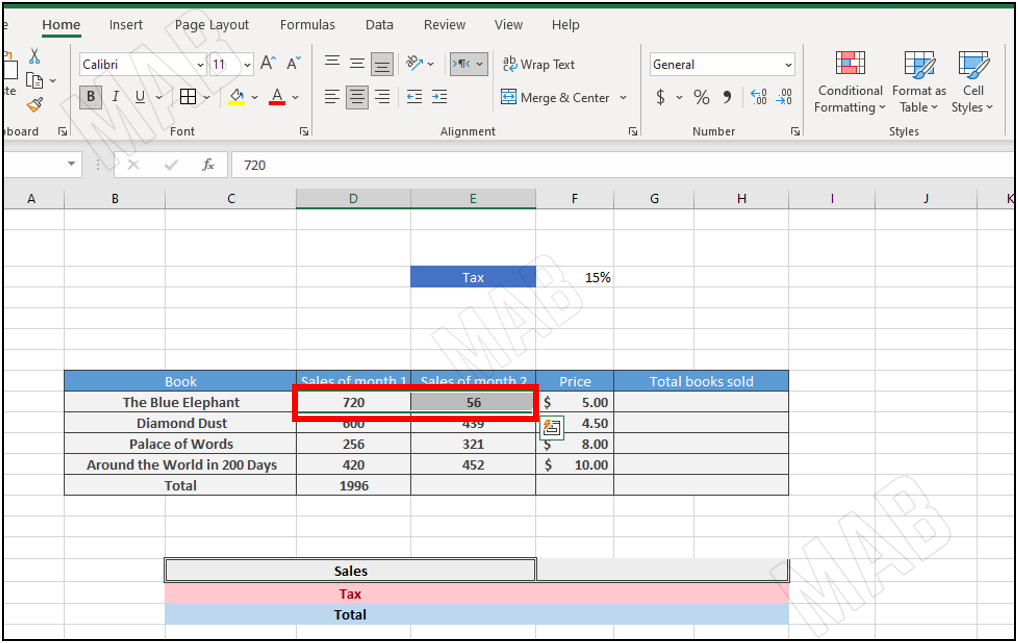
• Then from the toolbar we choose “Formulas” and then choose “Define Name”.
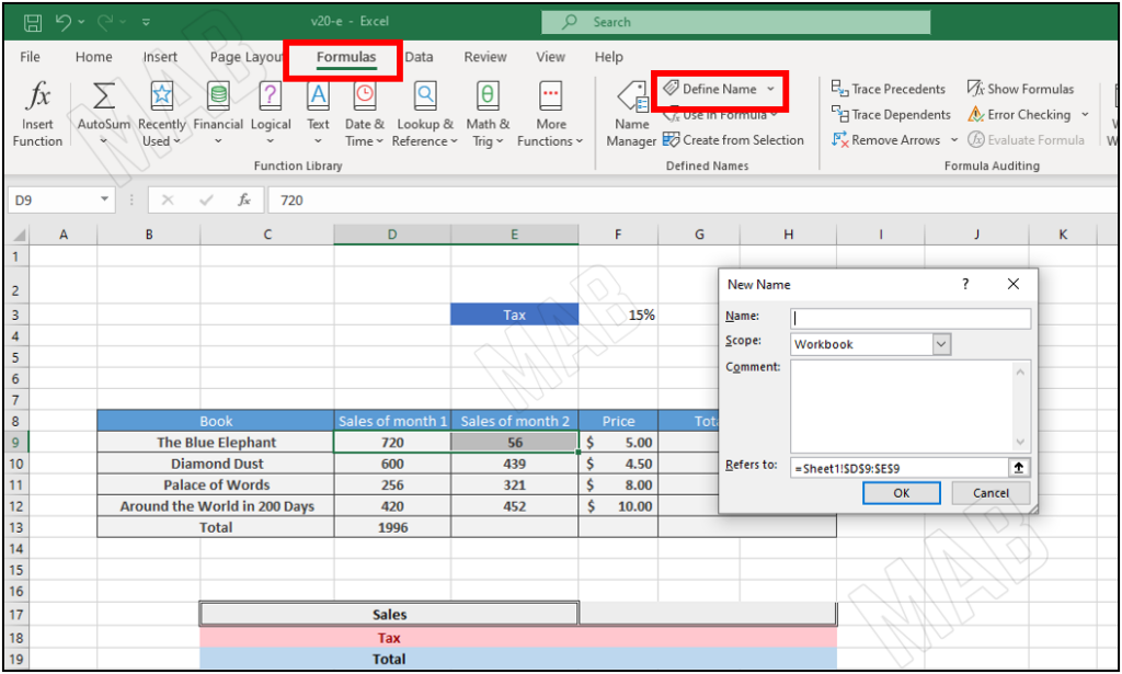
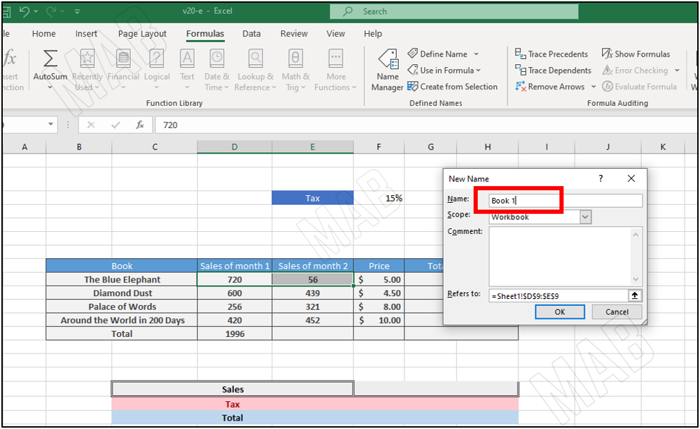
• We must also write the name we want, and in our example, we will write “Book1”, and then click “Ok”.
• Then from the toolbar and from “Formulas” as well, we choose “Name Manager”.
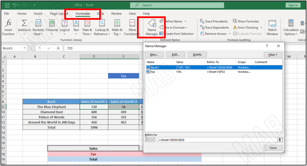
• From it we will notice the two names that we have given to the cells, and in our example they are: “Tax” and “Book 1”.
doing the sum based on the cells names
Now if you want to sum the books sold based on the names of the cells named using name manager, we will follow the following steps:
• First, we select the cell in which we want to put the sum result and then write the sum function “SUM=(“.
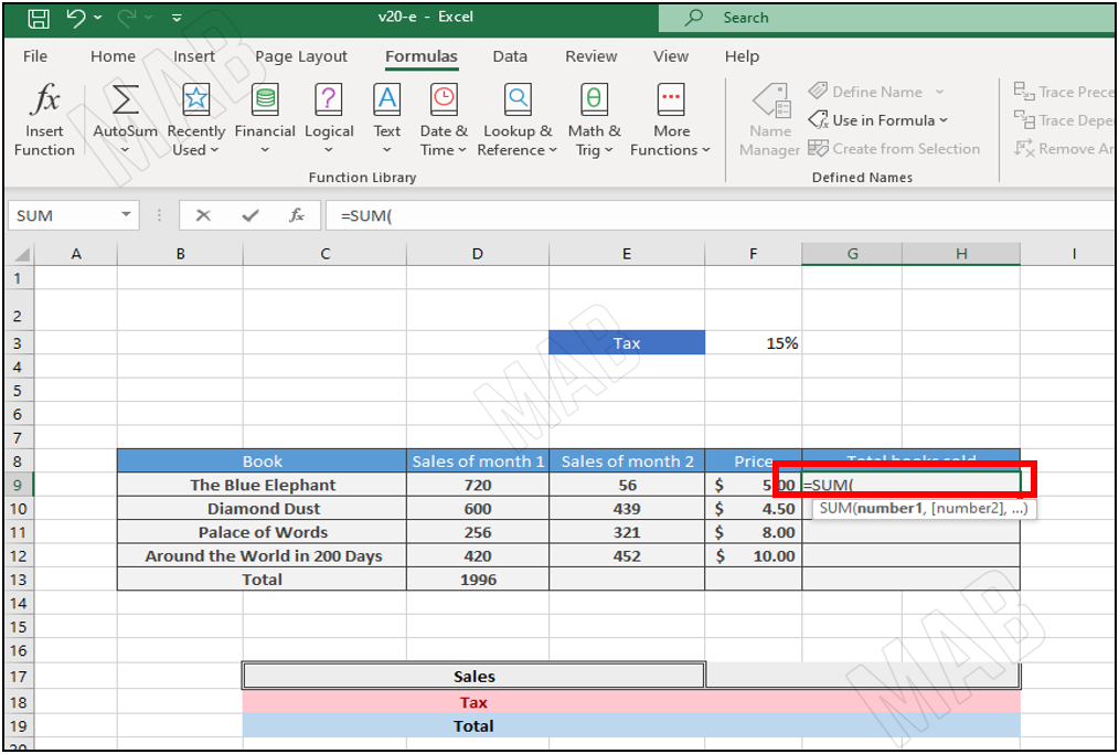
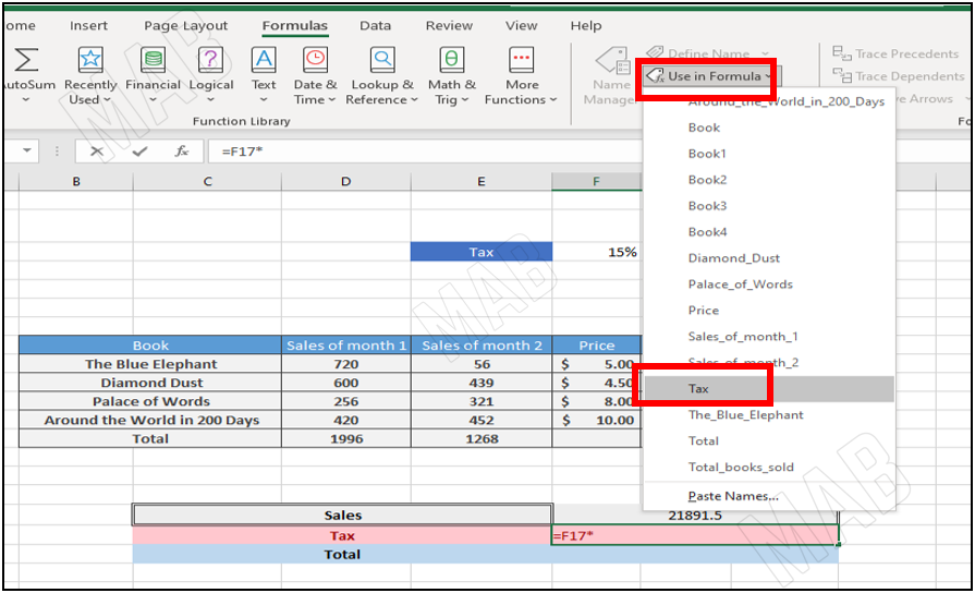
• Then from the toolbar we choose “Use in Formula”, and from it we select the name of the cells to which we want to apply the sum operation, then we choose “Ok”.
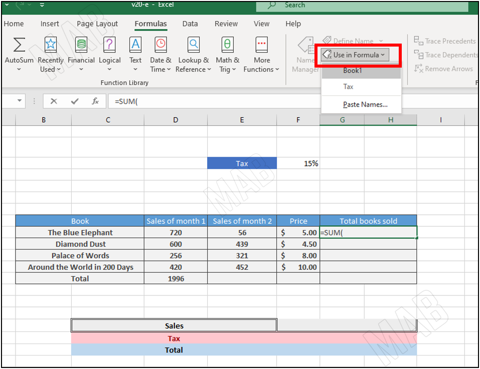
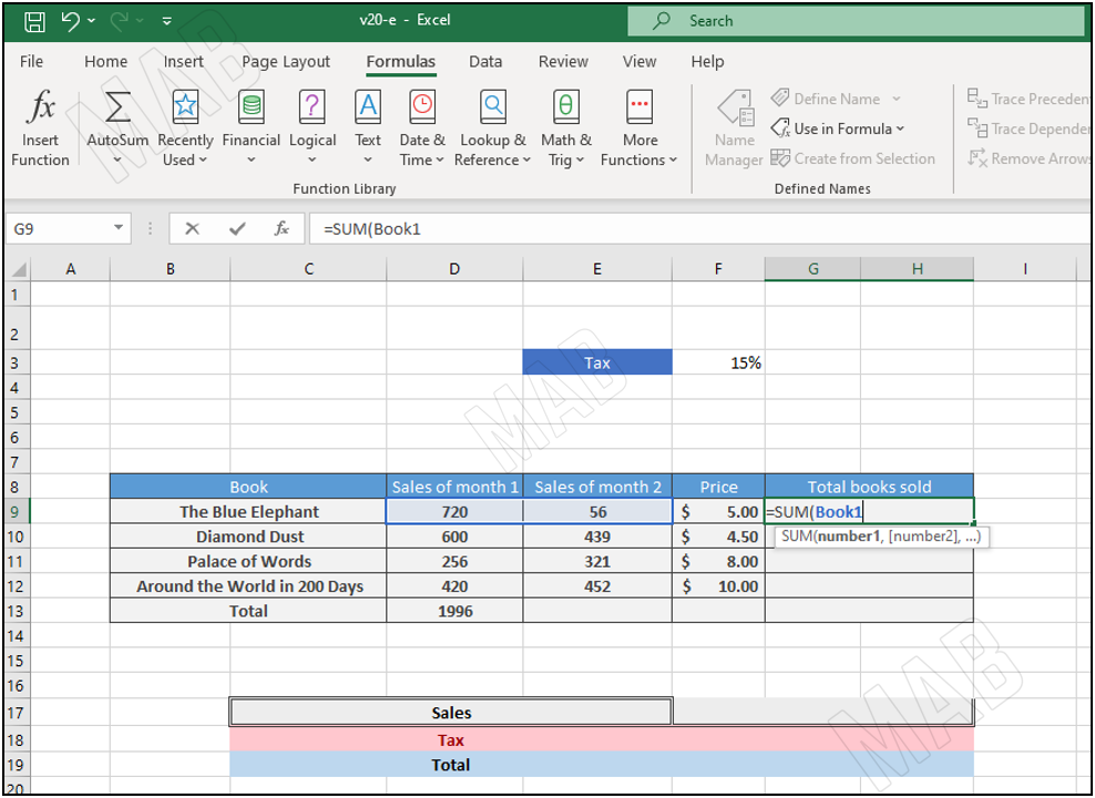
• Finally, we close the sum operation bracket and press “Enter” and the result of the operation appears.
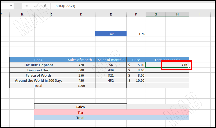
Note: If we drag down to apply the operation to all cells, the result will be a copy operation of the result only.
To apply the operation to all cells, we follow the following steps:
• First, we select all the numbers for the sales of the first and second months, with the names of the books.
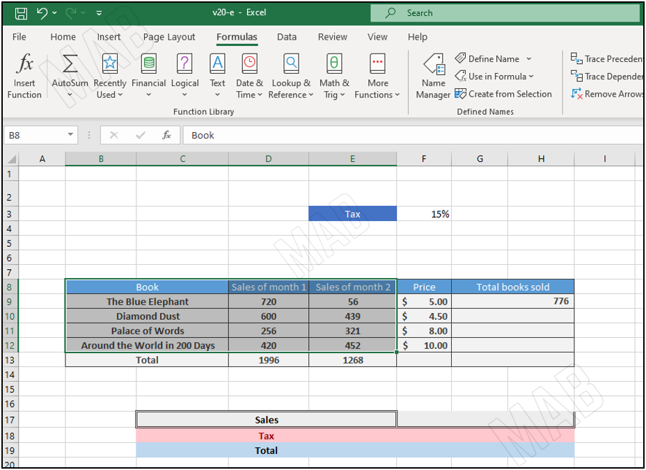
• Then from the toolbar and from “Formulas” we choose “Create From Selection”.
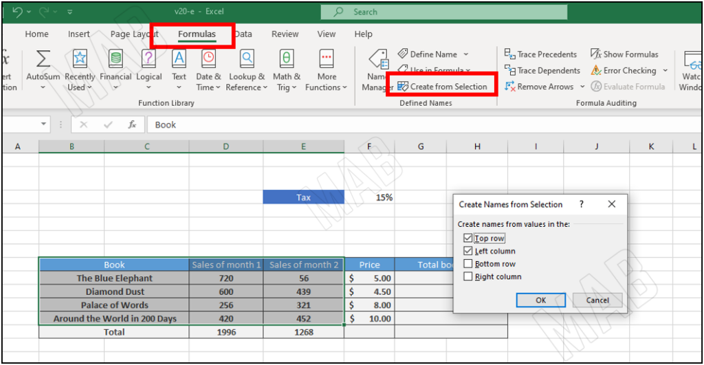
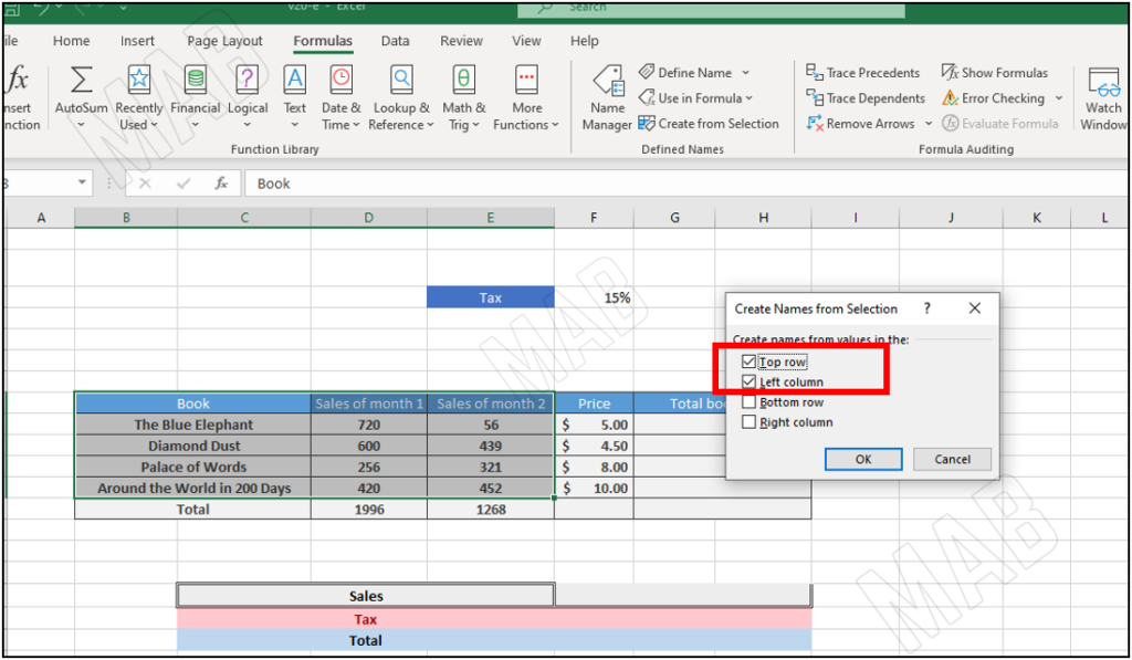
From it we choose the name of the cells, and how we want it to be determined. In this example, we will choose that the name be determined in the left column (which forms the names of the books), in addition to the first row (which expresses the number of the month of sales).
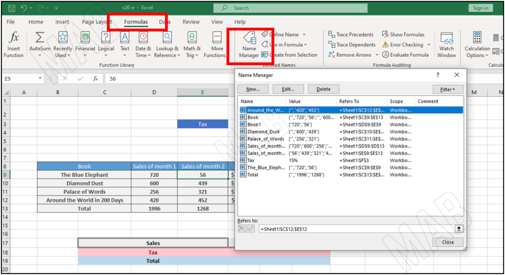
From the toolbar and also from “Formulas”, we choose “Name Manager”, and we notice how all the names have become abbreviations.
Calculating the total sales of the first month
Now, assuming that we want to calculate the total sales of the first month, we do the following steps:
• First, we select the cell in which we will put the summation result and write the summation function “Sum=(“.
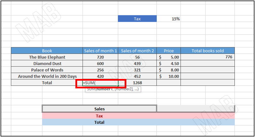
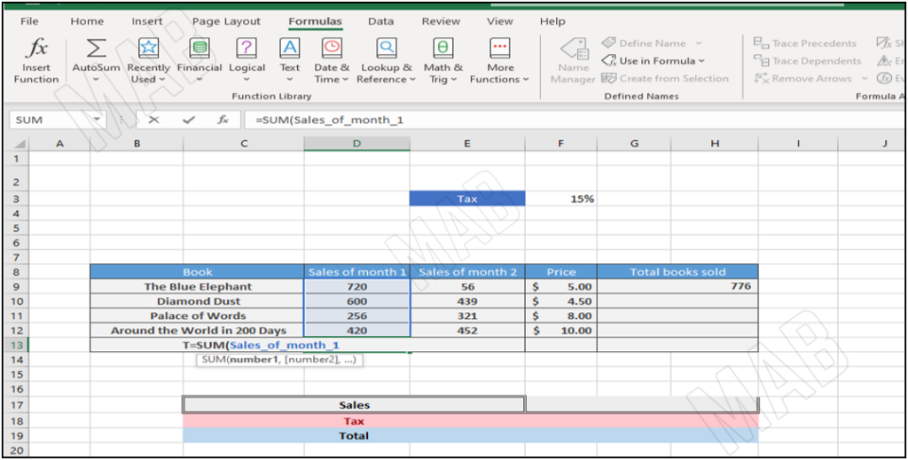
• Then from the “Use in Formula” toolbar, we specify the name of the cells to which we want to apply the summation operation and choose “Ok”. In our example, we will apply the summation operation to the sales of month 1.
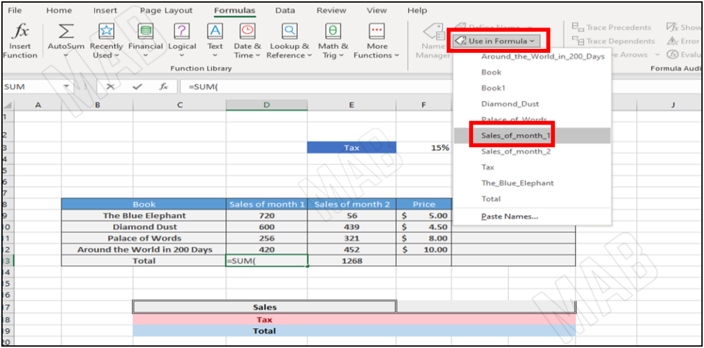
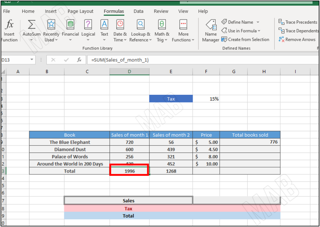
Finally, we close the bracket for the summation operation and press “Enter”, and notice how the summation result appears.
Now to calculate the total sales for all books, we will do the following steps:
• First, we calculate the sales for each book using the same previous method.
• Second, we select the sales of all books.
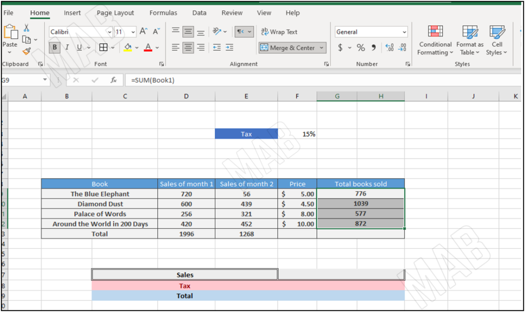
• Then from the toolbar, we choose “Define Name”.
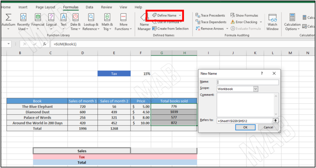
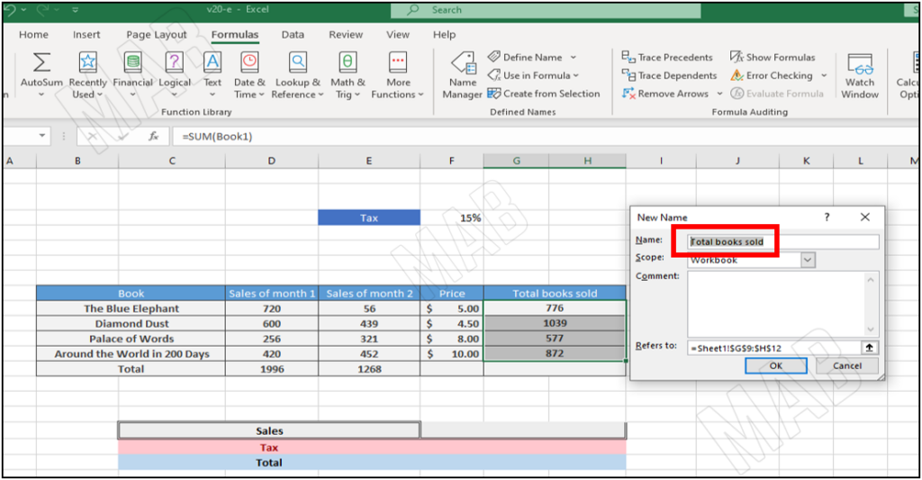
• A banner appears in which we write the name we want to express the selected information. In our example, we will leave the name as it is “Total Books Sold”, and then press “Ok”.
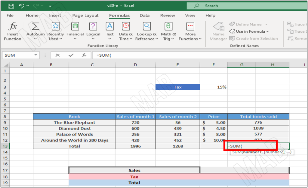
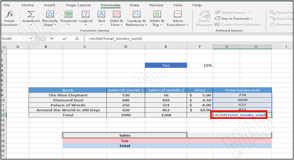
• We also select the cell in which we will put the summation result, and write the summation function “SUM(=”.
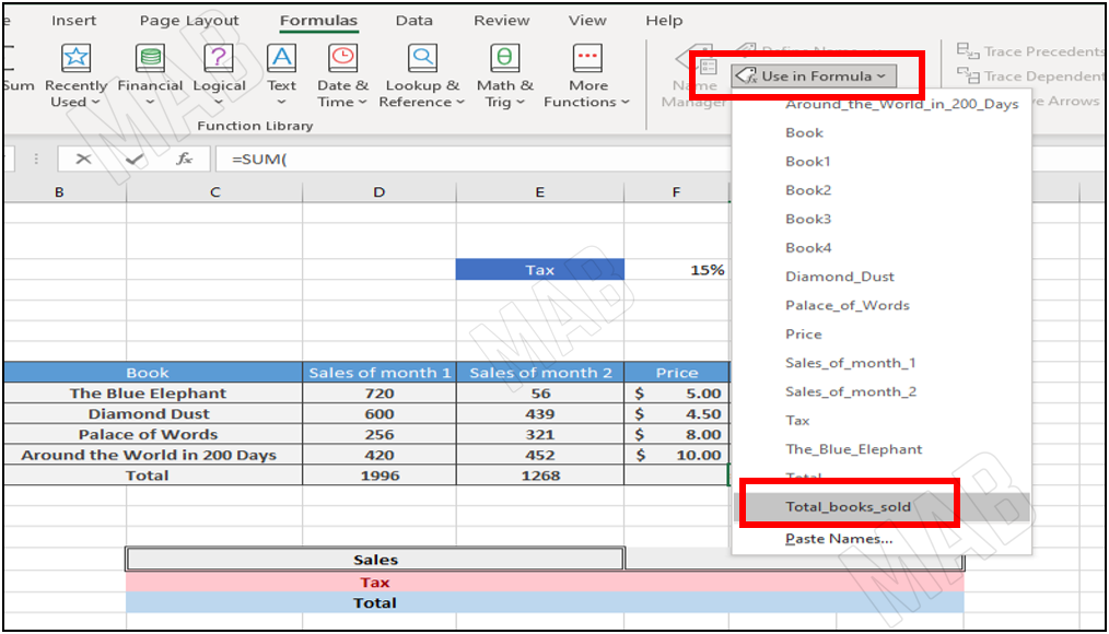
• Then from the toolbar we choose “Use in Formula”, specify the name of the cells to which we want to apply the summation operation, and choose “Ok”. In this example, we will apply the summation operation to “Total of Books Sold”.
• Finally, we close the bracket for the summation function and then press “Enter”, and the summation result appears.
Calculating the total sales
Now to calculate the total sales we must multiply the total number of books sold by the price, and to do this task we have the following steps:
• First, we select the cell on which we will perform the multiplication operation.
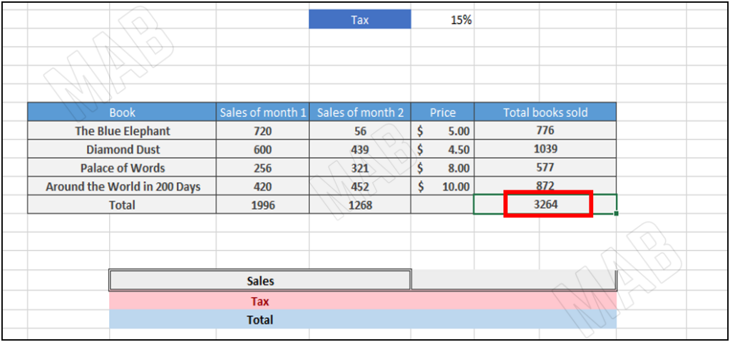
• Second, we click on this cell and then put the multiplication sign “*”.
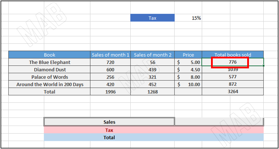
• Then we select the cell with which we will perform the multiplication operation.
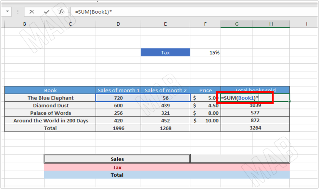
• We press “Enter”.
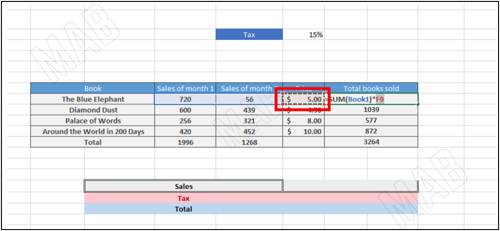
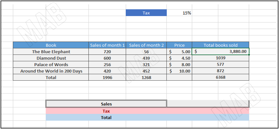
• Then we drag down to apply the operation to all other elements.
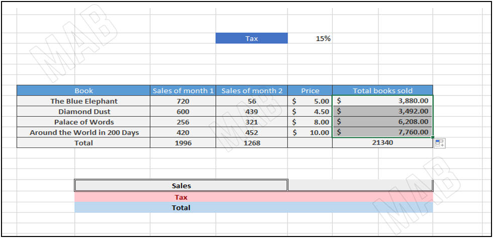
But the operation is not accurate as we must change the name of the element on which we apply the operation each time.
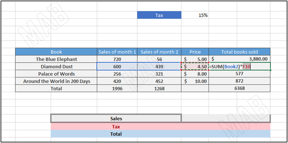
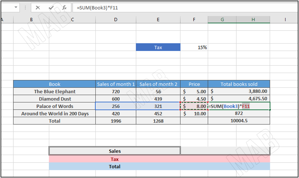
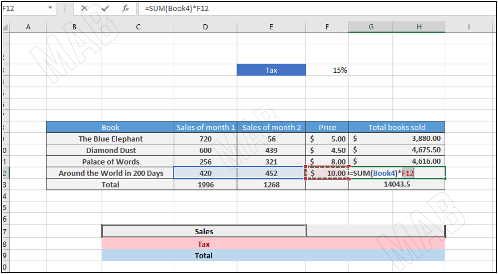
Thus, the final result is as follows:
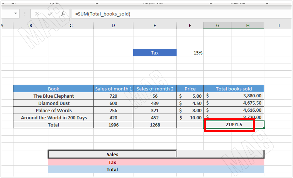
Calculating the sales
Now to calculate the sales, we will do the following steps:
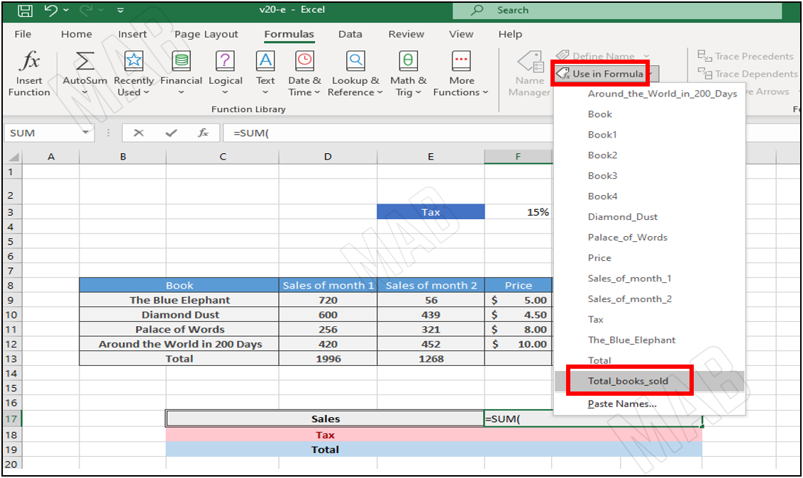
• First, we use the name “Total Books Sold”, again in the “Sales” box with the summation function “SUM(=” to calculate the sales again.
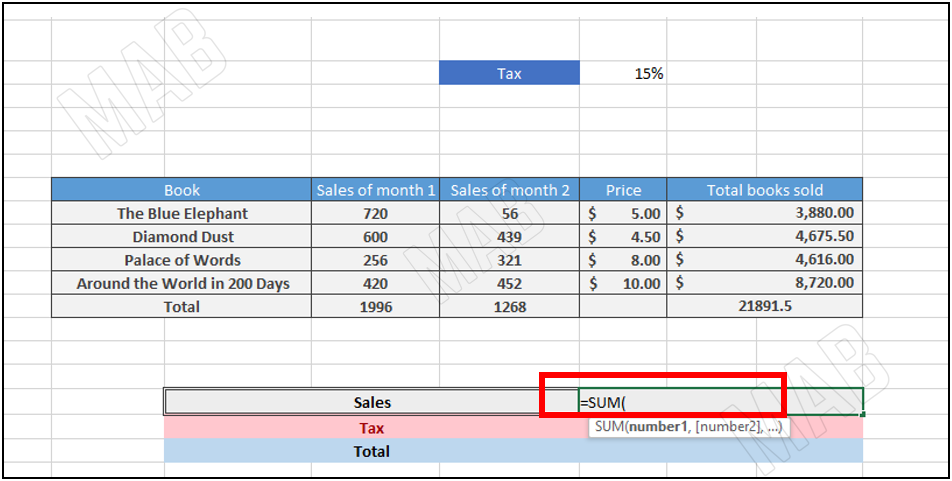
This is done by placing the summation function in the cell in which we want to put the result of the operation.
Then from the toolbar we choose “Formulas”, from it, we choose “Use in Formula”, and from the options we will choose “Total Books Sold”.
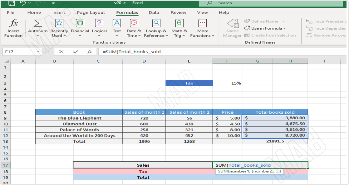
Then we close the bracket for the function and press “Enter”.
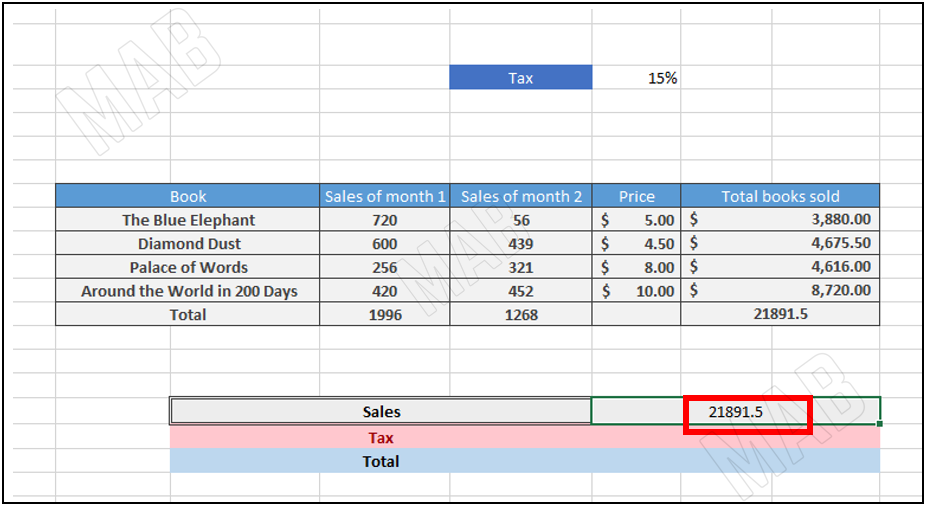
And thus we got the total again.
Calculating Tax with the Help of Name Manager
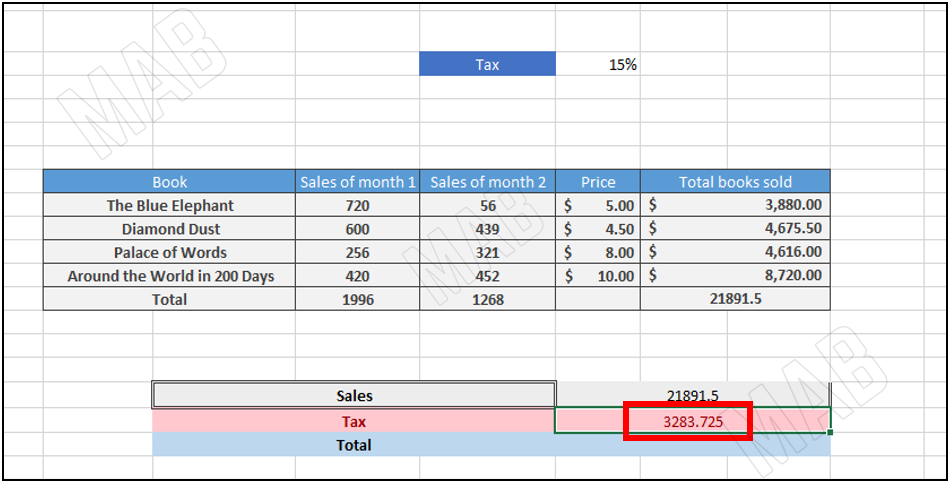
Now to get the tax we will multiply this sum with the cell for the tax which we gave the name “Tax”.
So we will follow the following steps:
• We specify the box in which we will put the result of the multiplication operation and write the sign “=”.
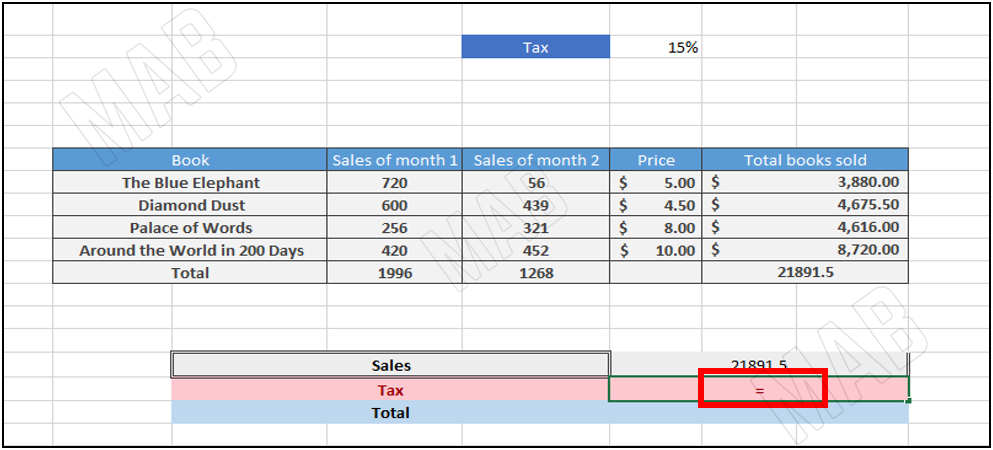
• We select the first cell that will enter into the multiplication operation which is the cell in which we put the sales result, and then we put the multiplication operation sign “*”.
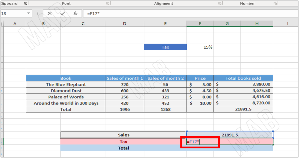
• We specify the second cell that will enter into the multiplication operation, and since we have previously added a name to the cell in “Name Manager”, then from the toolbar and from “Formula Use in”, we will choose “Tax”.
• From the keyboard we press “Enter”.
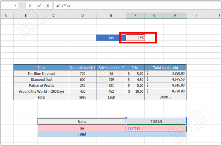
We will notice that the tax has been calculated.
Dear reader, if you liked the article, do not forget to subscribe to our YouTube channel, which provides all new in the field of technical and completely free training courses.
You can also browse our website to access the blog and read technical topics, or learn about the training courses offered by the site.
To access the full course “Excel Course” on YouTube, click here.


