In this lesson, we will learn two ways to apply automatic summation in Excel, which saves the time and effort required to calculate the sum of a large number of values.
The first method for automatic summation in Excel
Suppose that we have a large set of data in Excel, arranged as follows:

And we want the total sales of books sold during the weeks in the “Total Books Sold” cell, we do the following steps:
1- First, we select the cell in which we will place the summation operation (which is the “Total Books Sold” cell).

2- Second, we must write the summation function “=sum(” inside this cell.

3- After that, we select the cells that we will sum together by selecting and dragging on the cells we want.
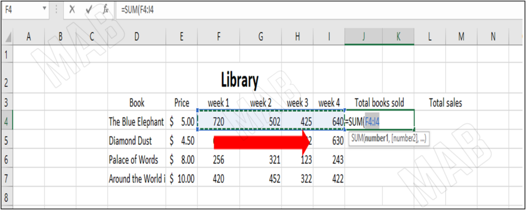
4- Then we close the bracket for the “sum” function.
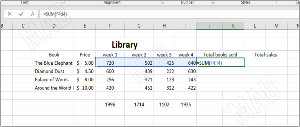
5- Finally, we press “Enter” and the summation result will appear.
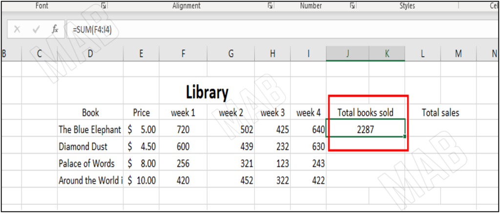
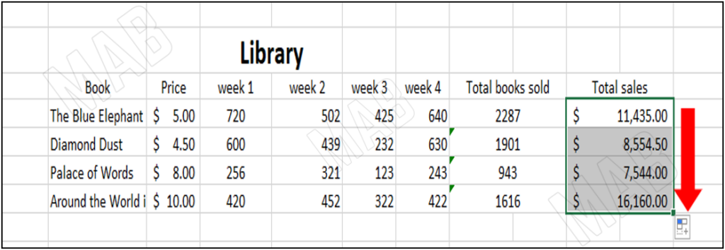
6- To apply the operation to all the values of the books, we will apply automatic summation, we will select and then drag starting from the cell in which we placed the summation operation downward.

calculate the total sales for the first book
Suppose we want to calculate the total sales for the first book, as we know we will multiply the price of the book by the total sales, through the following steps:
1- First, we put the “=” sign in the cell in which we want to put the multiplication operation, and then we select the cell of the resulting sum.

2- After that we put the multiplication operation symbol in this cell.

3- Then we select the cell with which we will perform the multiplication operation, which represents the price of the book.

4- Finally, we press “Enter” and the result appears.

5- It is also possible by selecting the first cell and dragging it down to apply the same operation to all cells in a similar manner.
The second method
1- First, from the toolbar, we choose “Home” and then “AutoSum”.
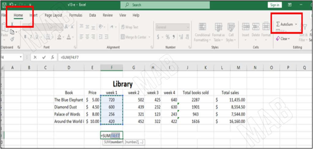
2- Then we notice that Excel has selected the group of cells, but there is an empty cell, so we change the selection by dragging to include only the cells that contain values.
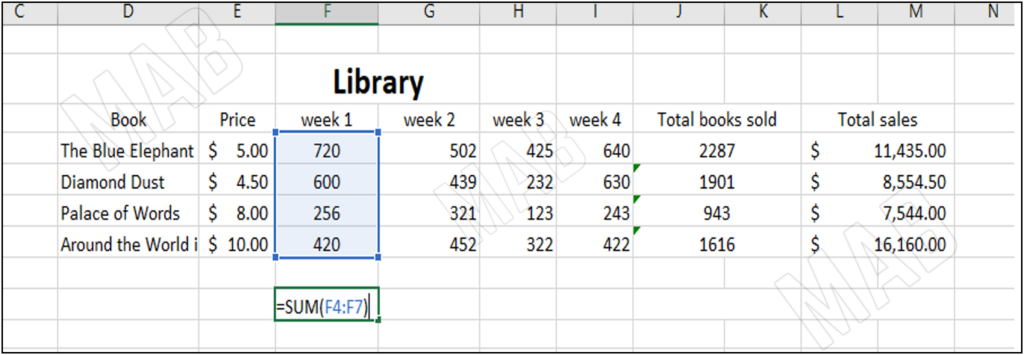
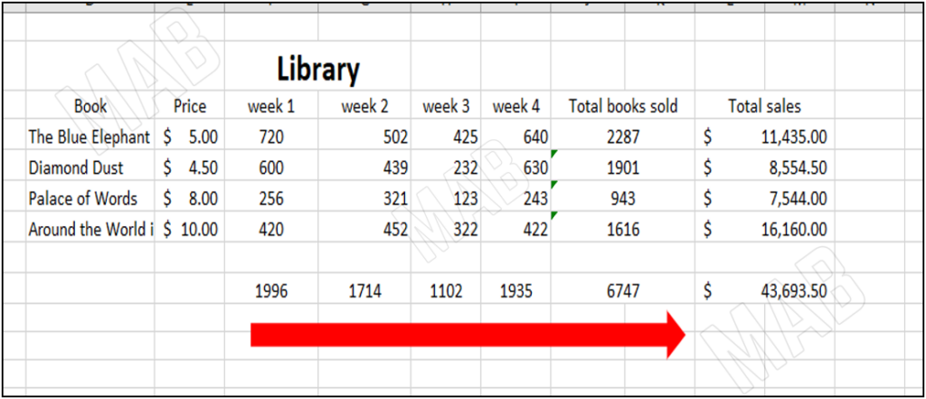
3-Then we press “Enter” and we notice the result appearing.

4- By dragging horizontally on all adjacent empty cells, we notice that the process has been applied to all cells.
Dear reader, if you liked the article, do not forget to subscribe to our YouTube channel, which provides all new in the field of technical and completely free training courses.
You can also browse our website to access the blog and read technical topics, or learn about the training courses offered by the site.
To access the full course “Excel Course” on YouTube, click here.


