In this lesson, we will learn How to Compare two columns of information in an Excel table. so we can distinguish different elements in a table with different colors.
Let us have the following two columns.
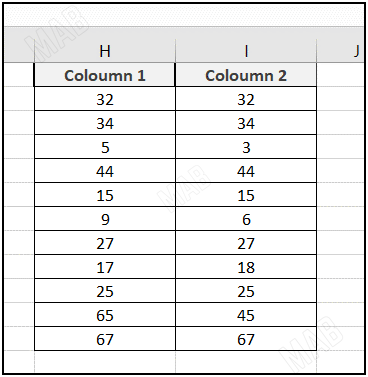
Suppose we want to distinguish different corresponding elements of the table with different colors.
To do this task, we will follow the following steps:
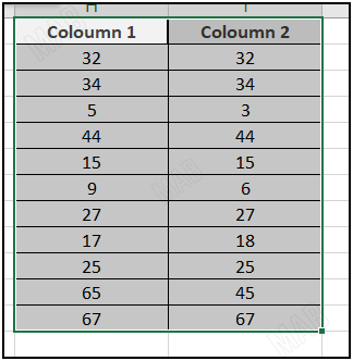
- We select the entire table.
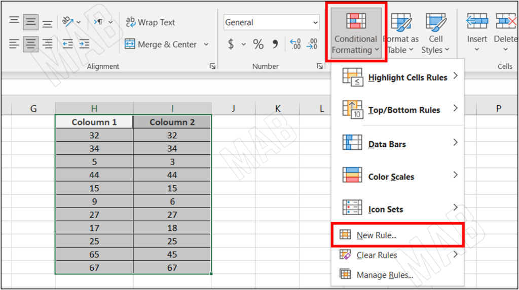
From the toolbar and from “Home” we choose “Conditional Formatting”, from which we will choose “New Rule”.
An interface will appear, and we will choose the last option “Use a Formula to determine which cells to format”.
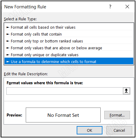
Now according to the option, we will determine what condition the cells are colored in, and to determine this condition within the empty rectangle we will do the following:
- We write the sign “=”.
- Then, We select the first cell of the first column.
- We write the sign “<>” which means not equal.
- We select the first cell of the second column.
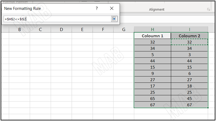
We remove the key sign next to the cell numbers so that the operation is applied to the entire two columns instead of applying it to the two selected cells only.
We get the following form: =$H2<>$I2

From “Format” and then “Fill” we can choose the color of the different cells.
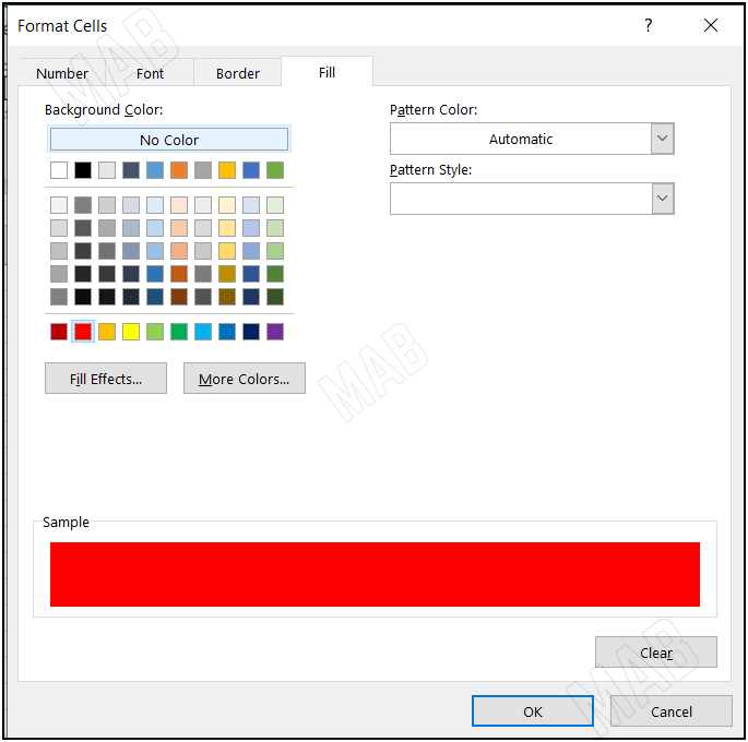
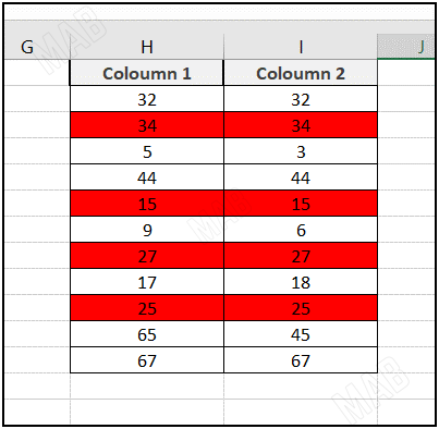
Here we will choose the red color and then choose “Ok”, so the different opposite cells appear in red.
Dear reader, if you liked the article, do not forget to subscribe to our YouTube channel, which provides all new in the field of technical and completely free training courses.
You can also browse our website to access the blog and read technical topics, or learn about the training courses offered by the site.
To access the full course “Excel Course” on YouTube, click here.


