In this lesson, we will learn the mechanism of cumulative summation in Excel to add a large set of values quickly and easily.
How to use cumulative summation, suppose we have sales for a whole week totaling 205, but I want to see in detail the sales of one day and the days that come before it during the week.
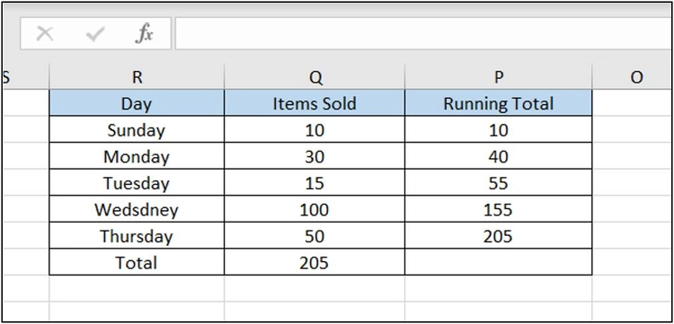
Running total step by step
1- First, we put an equal sign “=”.
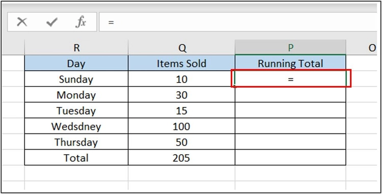
2- Second, we select the cell that contains the first number, which is “10”.
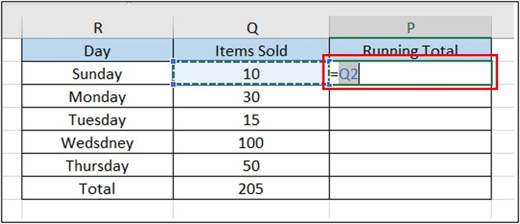
3- Then from the keyboard we choose “Enter”.
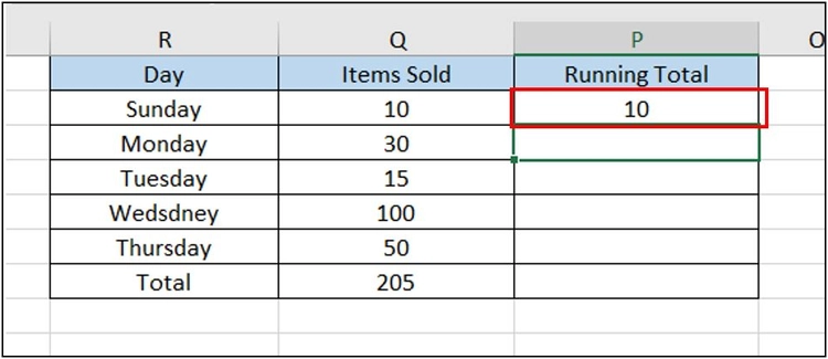
4- After that, we move to the cell below the previous cell and put an “=” sign.
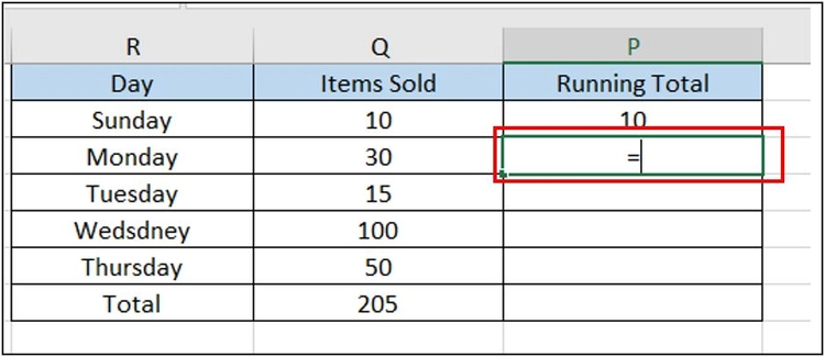
5- Then we select the new cell that contains the number “10”.
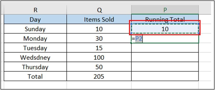
6- We put a “+” sign.
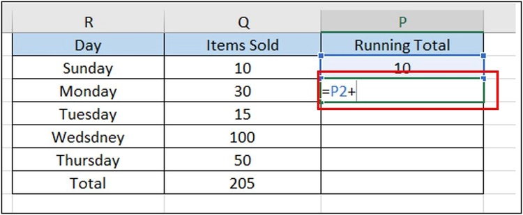
7- Then we select the cell that follows the old cell that contains the number “10”, which is the cell that contains the number “30”.
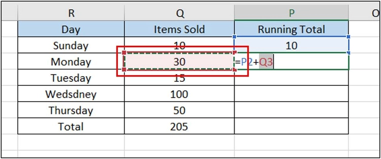
8- we choose “Enter”, From the keyboard.
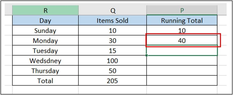
9- We drag from this cell towards the cells below it, and we notice that the same process has been applied to all other cells.
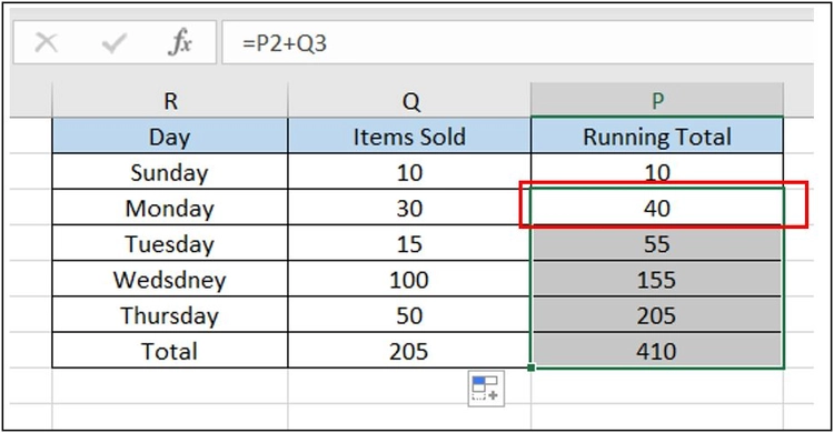
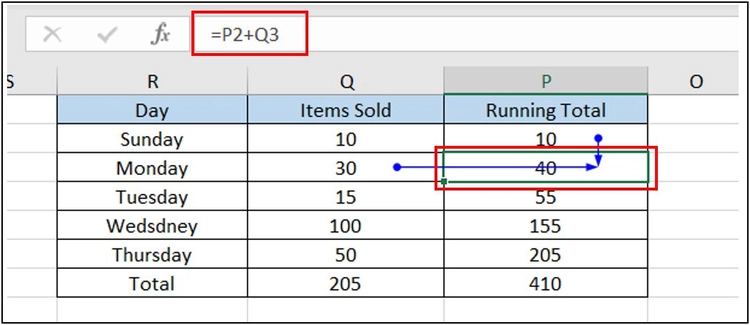
Then we select the second cell and from the toolbar and from “Formulas” we choose “Trace Precedents”. This way we can see the details of the mathematical operation and the values used in the operation.
Dear reader, if you liked the article, do not forget to subscribe to our YouTube channel, which provides all new in the field of technical and completely free training courses.
You can also browse our website to access the blog and read technical topics, or learn about the training courses offered by the site.
To access the full course “Excel Course” on YouTube, click here.


